每个概念先解释再用,配一个算例或一个可玩的动画。Every concept is explained before use, with a worked example or a playable animation.
物理与统计:从零到 DET_MLPhysics & Statistics: From Zero to DET_ML
这一页把项目用到的所有统计概念从微积分和基本概率的水平搭起来。你不需要预先知道泊松似然、Cash 统计量、Wilks 定理或 χ² 分布。This page builds all the statistical concepts the project uses from the level of calculus and basic probability. You do not need to know the Poisson likelihood, the Cash statistic, Wilks' theorem, or the χ² distribution beforehand.
1. 光子是数出来的1. Photons Are Counted
X 射线探测器不像普通相机那样测"亮度",它是一个一个地数光子。一块天空区域的平均光子率是 λ(比如每像素 0.05 个),但任何一次观测里实际数到的数目 Y 是随机的。这个随机性的规律就是泊松分布(Poisson distribution):An X-ray detector does not measure "brightness" like a normal camera; it counts photons one by one. A patch of sky has an average photon rate λ (say 0.05 per pixel), but the actual count Y in any single observation is random. The rule for that randomness is the Poisson distribution:
P(Y = k | λ) = λᵏ e^(−λ) / k! 均值 = 方差 = λ
"均值 = 方差"是泊松统计的核心:数到 100 个光子,涨落就是 √100 = 10 个。数得越多,相对涨落越小。这就是为什么亮源好测、暗源难测。"Mean = variance" is the core of Poisson statistics: if you count 100 photons, the fluctuation is √100 = 10. The more you count, the smaller the relative fluctuation. That is why bright sources are easy to measure and faint ones are hard.
动画 1:泊松光子落到像素网格上。拖动"源强度 S"和"背景 b"滑块,看图像怎么变;点"再随机一次"换一批光子。注意:即使 S = 0,背景也会随机地在某些像素上堆出几个光子。Animation 1: Poisson photons landing on a pixel grid. Drag the "Source strength S" and "Background b" sliders to see how the image changes; press "Re-roll photons" for a new photon draw. Note: even with S = 0, the background randomly piles up a few photons in some pixels.
来源:本页动画用 lib/simulate.py 的同一模型(Y ~ Poisson(b + S·P)),种子固定;静态对照图见下图。Source: the animation on this page uses the same model as lib/simulate.py (Y ~ Poisson(b + S·P)), fixed seed; a static comparison image is shown below.
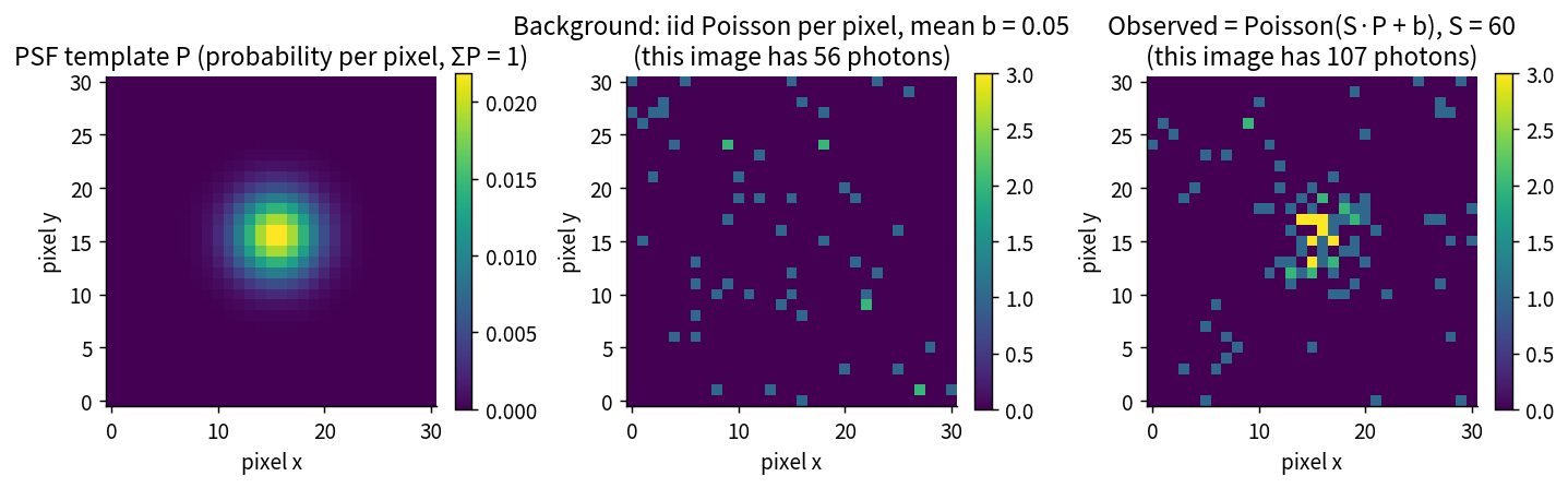
来源:scratchpad/v2/T12/make_figures.py(lib/simulate.py,S=60,b=0.05,种子 42)。Source: scratchpad/v2/T12/make_figures.py (lib/simulate.py, S=60, b=0.05, seed 42).
2. PSF:一个源的光子落在哪儿2. PSF: Where a Source's Photons Land
望远镜不是完美的:一个点源的光子不会全落在一个像素上,而是散开成一个小光斑。这个光斑的形状叫点扩散函数(point spread function, PSF)。XMM-Newton 的 PSF 半功率直径约 15 角秒,相当于约 4 个像素(每像素 4 角秒)。A telescope is not perfect: a point source's photons do not all land in one pixel; they spread into a small spot. The shape of that spot is called the point spread function (PSF). XMM-Newton's PSF has a half-power diameter of about 15 arcsec, which is about 4 pixels (4 arcsec per pixel).
我们把 PSF 写成归一化的模板 P:第 i 个像素上 Pi 是"源的一个光子落在这里"的概率,ΣPi = 1。于是一个总流量为 S 的源在第 i 个像素上贡献的平均光子数是 S·Pi,再加上背景 b(每像素),该像素的期望计数是:We write the PSF as a normalized template P: the value Pi at pixel i is the probability that "a source photon lands here", with ΣPi = 1. A source with total flux S contributes an average of S·Pi photons to pixel i; adding the background b (per pixel), the expected count in that pixel is:
μᵢ = b + S·Pᵢ
这就是全项目唯一的数据模型:每个像素独立泊松,均值 μᵢ = b + S·Pᵢ。This is the project's only data model: each pixel is independent Poisson with mean μᵢ = b + S·Pᵢ.
真实的 XMM PSF 不是高斯,是带翼的 ELLBETA 模型(King 轮廓 + 高斯核),而且随能量、离轴角、方位角变化。项目的 Stage 1 先用高斯 PSF 把统计规律搞清楚,Stage 2 才换上真实模板。这一段历史见历史页。The real XMM PSF is not Gaussian; it is a winged ELLBETA model (King profile + Gaussian core) and varies with energy, off-axis angle, and azimuth. Stage 1 of the project used a Gaussian PSF to get the statistics clear; Stage 2 switched to the real templates. That history is on the History page.
3. 似然与 Cash 统计量3. Likelihood and the Cash Statistic
给定模型参数(比如源的流量 S),"数据有多可能出现"叫似然(likelihood)。对独立泊松像素,联合似然是每个像素的泊松概率相乘。取对数后变成求和:Given the model parameters (say the source flux S), "how likely is the data" is called the likelihood. For independent Poisson pixels, the joint likelihood is the product of each pixel's Poisson probability. Taking logs turns it into a sum:
ℓ(S) = Σᵢ [ Yᵢ ln μᵢ(S) − μᵢ(S) ] μᵢ(S) = b + S·Pᵢ
最大似然拟合(maximum likelihood fit)就是找让 ℓ 最大的 S。天文上习惯用 Cash 统计量(Cash statistic):Maximum likelihood fitting is finding the S that maximizes ℓ. Astronomers conventionally use the Cash statistic:
C(S) = −2ℓ(S) + 常数 = 2 Σᵢ [ μᵢ(S) − Yᵢ ln μᵢ(S) ]
C 越小,似然越大。所以拟合 = 把 S 滑到 C 最小的地方。Smaller C means larger likelihood. So fitting = sliding S until C is minimum.
动画 2:拖动"试探单源振幅 S"滑块,看 Cash 统计量 C(S) 怎么变。红色虚线是"只有背景"的模型(S = 0)的 C_null;绿色箭头的高度就是 ΔC。点"自动拟合到最小"看拟合器做什么;点"换一张新图像"换一批光子再做一次。Animation 2: drag the "Trial source amplitude S" slider to see how the Cash statistic C(S) changes. The red dashed line is the C_null of the "background-only" model (S = 0); the green arrow's height is ΔC. Press "Auto-fit to the minimum" to watch the fitter work; press "New image" for a new photon draw and re-fit.
来源:动画内嵌的泊松模拟与 lib/fit.py 的 cash_statistic 完全一致(C = 2Σ(μ − Y ln μ))。Source: the embedded Poisson simulation and lib/fit.py's cash_statistic are identical (C = 2Σ(μ − Y ln μ)).
4. ΔC:似然比统计量4. ΔC: The Likelihood-Ratio Statistic
"这个源是真的还是背景涨落?"用似然比(likelihood ratio)回答:比较"只有背景"的模型(零假设)和"背景 + 一个源"的模型谁更可能。用 Cash 统计量写出来就是:"Is this source real or a background fluctuation?" The answer uses the likelihood ratio: compare the "background-only" model (null hypothesis) with the "background + one source" model. In Cash-statistic terms:
ΔC = C_null − C_min ≥ 0
ΔC 越大,说明"有源"比"没源"好得越多。它就是 emldetect 内部真正计算的检测统计量。The larger ΔC, the more "source present" beats "no source". It is the actual detection statistic computed inside emldetect.
算例(动画 2 里的那张图):S_true = 25 counts,b = 0.05/像素。拟合找到 Ŝ ≈ 24.6,C_min ≈ 928.4,C_null ≈ 948.9,所以 ΔC ≈ 20.5。这个 ΔC 对应的 DET_ML ≈ 8.9(下一节讲怎么换算)——刚过 6–10 窗口的中部。Worked example (the image in Animation 2): S_true = 25 counts, b = 0.05/pixel. The fit finds Ŝ ≈ 24.6, C_min ≈ 928.4, C_null ≈ 948.9, so ΔC ≈ 20.5. That ΔC corresponds to DET_ML ≈ 8.9 (next section explains the conversion) — right in the middle of the 6–10 window.
注意 ΔC 是拟合完之后才有的量:拟合器先找到最好的 S(和位置),才有 C_min。这一点后面会反复重要:拟合本身会"吸收"一部分背景涨落,让 ΔC 比朴素理论预期的大。Note that ΔC only exists after the fit: the fitter first finds the best S (and position), and only then is C_min available. This point matters repeatedly: the fit itself "absorbs" some of the background fluctuation, making ΔC larger than the naive theory predicts.
为什么"探测即真"在可观空间里几乎精确。在拟合幅度处,模型计数 ê 与数据 n 满足极大似然的得分方程:残差 (n − ê) 与模板 P/ê 正交。于是观测差 ΔC_obs − ΔC_A(Ŝ) = 2Σ(n−ê) ln(1+ŜP/b) 在一阶上消失——把 Ŝ 当作已知量去算 ΔC,与拿它当自由参数的拟合结果,差别只剩二阶项:δ(条件均值的二阶修正:拟合幅度的涨落经过 ΔC 的曲率带来的偏移)和 V(方差项)。这让在可观测量 (Ŝ, b) 上做条件理论变得很自然,但本项目仍然用模拟去检验它——一阶消失是数学,二阶项的大小是物理。Why "detected = true" is nearly exact in observable space. At the fitted amplitude the model counts ê and the data n satisfy the maximum-likelihood score equation: the residual (n − ê) is orthogonal to the template P/ê. So the observed difference ΔC_obs − ΔC_A(Ŝ) = 2Σ(n−ê) ln(1+ŜP/b) vanishes to first order — computing ΔC with Ŝ treated as known gives the same answer as the free-parameter fit, up to second-order terms: δ (the second-order correction to the conditional mean: the shift that fluctuations of the fitted amplitude produce through the curvature of ΔC) and V (the variance term). This makes conditional theory on the observables (Ŝ, b) natural, but the project still tests it with simulations — the first-order vanishing is mathematics; the size of the second-order terms is physics.
5. Wilks 定理与 χ²:什么时候能用,什么时候不能5. Wilks' Theorem and χ²: When It Works and When It Doesn't
统计学里有一条很方便的定理(Wilks 定理,1938):如果数据量足够大、参数都在定义域内部、模型正确,那么 ΔC 近似服从 χ² 分布(chi-square distribution),自由度 ν 等于多出来的参数个数。Statistics has a handy theorem (Wilks' theorem, 1938): if the data are plentiful, all parameters are in the interior of their domains, and the model is correct, then ΔC approximately follows a χ² (chi-square) distribution with degrees of freedom ν equal to the number of extra parameters.
我们的单源拟合有 3 个自由参数:流量 S、位置 x、位置 y。所以朴素的想法是 ν = 3,ΔC ~ χ²₃。但这里有 2 个"非标准"的地方:Our single-source fit has 3 free parameters: flux S, position x, position y. The naive guess is ν = 3, so ΔC ~ χ²₃. But there are 2 "non-standard" features:
- 边界:S 不能是负的。没有源时 S_true = 0 正好在边界上,约一半的纯背景图像拟合出 Ŝ = 0,ΔC = 0。所以零分布是"一半质量在 0 + 尾部 ≈ ½χ²₁",而不是 χ²₃。Boundary: S cannot be negative. When there is no source, S_true = 0 sits exactly on the boundary; about half of pure-background images fit to Ŝ = 0 with ΔC = 0. The null distribution is therefore "half the mass at 0 + a tail ≈ ½χ²₁", not χ²₃.
- 位置在零假设下不可识别:"没有源"时谈"源的位置"没有意义,这让位置自由度不能简单地算进 ν。Position unidentifiable under the null: when there is no source, "the source's position" is meaningless, so the position degrees of freedom cannot simply count toward ν.
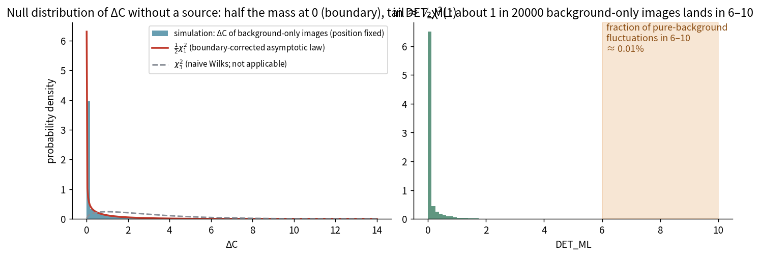
来源:scratchpad/v2/T12/make_figures.py(lib/fit.py 的 fit_amplitude_only,位置固定,b = 0.05,20000 次实现)。Source: scratchpad/v2/T12/make_figures.py (lib/fit.py's fit_amplitude_only, position fixed, b = 0.05, 20000 realizations).
这个教训是项目里反复出现的主题:渐近定理给出骨架,有限计数的修正必须靠模拟。论文里把这叫"beyond-Fisher"效应(见历史页的 E086–E096)。This lesson recurs throughout the project: the asymptotic theorem gives the skeleton; the finite-count corrections must come from simulation. The paper calls these "beyond-Fisher" effects (see the History page, E086–E096).
6. DET_ML:目录用的数6. DET_ML: The Catalogue's Number
emldetect 不直接报告 ΔC,而是把它换算成 DET_ML(detection maximum likelihood)。换算规则是 SAS 文档写死的:emldetect does not report ΔC directly; it converts it to DET_ML (detection maximum likelihood). The conversion rule is hard-coded in the SAS documentation:
DET_ML = −ln Q(ν/2, ΔC/2)
其中 Q 是上不完全伽马函数(upper incomplete gamma function),ν = n_images + 2(n 幅图像联合拟合时)。单幅图像 ν = 3。Q(3/2, ΔC/2) 就是"如果零假设为真,χ²₃ 超过 ΔC 的概率";取负对数后,DET_ML 越大表示越不可能是背景涨落。Here Q is the upper incomplete gamma function, and ν = n_images + 2 (when n images are jointly fitted). For a single image ν = 3. Q(3/2, ΔC/2) is "if the null is true, the probability that χ²₃ exceeds ΔC"; the negative log makes DET_ML larger when the signal is less likely to be a background fluctuation.
动画 3:拖动 ΔC 滑块,看它变成多少 DET_ML。橙色带是 4XMM 目录的 6–10 窗口(ΔC 14.34–22.76)。注意 ΔC 到 DET_ML 是非线性压缩:ΔC 翻倍,DET_ML 并不翻倍。Animation 3: drag the ΔC slider to see what DET_ML it becomes. The orange band is the 4XMM catalogue's 6–10 window (ΔC 14.34–22.76). Note the nonlinear compression: doubling ΔC does not double DET_ML.
来源:lib/detml.py 的约定(DET_ML = −ln Q(ν/2, ΔC/2),自然对数)。动画里的 Q 用连分式计算,与 scipy.special.gammaincc 一致。Source: lib/detml.py's convention (DET_ML = −ln Q(ν/2, ΔC/2), natural log). The animation computes Q via a continued fraction, matching scipy.special.gammaincc.
三个约定陷阱(违反会差 2 到 50 倍):Three convention traps (violating them causes 2 to 50 times errors):
- DET_ML 用自然对数 ln,不是 log10(差 ln 10 = 2.303 倍);DET_ML uses natural log ln, not log10 (factor ln 10 = 2.303);
- Q 的第二个参数是 ΔC/2,不是 ΔC(漏掉 /2 会把阈值算小一倍);Q's second argument is ΔC/2, not ΔC (dropping /2 halves the threshold);
- 目录里的
delta_c_nu3列存的是 ΔC/2,不是 ΔC(要乘 2)。The catalogue'sdelta_c_nu3column stores ΔC/2, not ΔC (multiply by 2).
来源:CLAUDE.md 的"Catalog Convention Traps (I041)"与 PITFALLS.md。Source: CLAUDE.md's "Catalog Convention Traps (I041)" and PITFALLS.md.
7. 铁律:不许按 ML 切样本7. The Iron Rule: No ML-Based Sample Cuts
项目有一条写进 CLAUDE.md 的 IRON RULE,违反它的分析全部作废:The project has an IRON RULE written into CLAUDE.md; any analysis violating it is void:
永远不要用 ML 或 DET_ML 来截取样本,再分析条件分布。条件化变量必须是可观测量 (Ŝ, b),不是 S_true,更不是 ML 本身。统计要在 ΔC 残差空间里做,不要直接在 ML 空间做。Never use ML or DET_ML to cut samples and then analyse conditional distributions. The conditioning variables must be the observables (Ŝ, b), not S_true, and certainly not ML itself. Statistics must be done in the ΔC residual space, not in ML space.
为什么?因为 ML 是 ΔC 的非线性变换,而 ΔC 又依赖 Ŝ。按"ML 在 6–10"切样本,相当于按一个和答案相关的量筛选数据——这叫选择偏差(selection bias),会把条件分布切歪。正确的做法是:Why? Because ML is a nonlinear transform of ΔC, and ΔC depends on Ŝ. Cutting samples by "ML in 6–10" means selecting data by a quantity that correlates with the answer — that is selection bias, and it distorts the conditional distribution. The correct procedure is:
- 按 Ŝ 分箱(不是按 ML);Bin by Ŝ (not by ML);
- 每个源减去理论预测的 ΔC 均值,得到残差 z = (ΔC_obs − μ_model) / σ_model;Subtract the theoretical mean ΔC from each source to get the residual z = (ΔC_obs − μ_model) / σ_model;
- 在残差空间里看均值、宽度、偏度;Inspect mean, width, skewness in the residual space;
- "DET_ML 6–10 的源"用"典型 DET_ML 落在 6–10 的 Ŝ 箱"来选,而不是按每个源的 ML 切。"Sources with DET_ML 6–10" are selected by "Ŝ bins whose typical DET_ML falls in 6–10", not by cutting on each source's ML.
这条规则是 2026-05 到 2026-09 多次踩坑后定下来的(见历史页的 T40、E151)。This rule was fixed after several stumbles from 2026-05 to 2026-09 (see the History page, T40 and E151).
8. Eddington 偏差:为什么测得的流量偏亮8. Eddington Bias: Why Measured Fluxes Are Biased High
天上暗源比亮源多得多。X 射线源的数目大致按 dN/dS ∝ S^−2.5 增长:流量每暗一倍(2 倍),数量多约 5.7 倍。现在加上泊松涨落:一个真实流量 5 counts 的源,测出来可能是 3 也可能是 8;一个真实 50 counts 的源,测出来 45 或 55。There are vastly more faint X-ray sources than bright ones. The number of sources roughly follows dN/dS ∝ S^−2.5: every factor of 2 fainter in flux means ~5.7× more sources. Now add Poisson scatter: a true 5-count source measures 3 or 8; a true 50-count source measures 45 or 55.
关键在于:从 5 涨落到 8 的源,比从 50 跌落到 8 的源多得多,因为 5 counts 的源本来就多。结果是在"测得 Ŝ = 8"的源里,混进了大量本来更暗的源。于是测得的流量系统性地偏亮——这就是 Eddington 偏差(Eddington bias),1913 年就由 Eddington 本人描述过。The key is: sources that scatter from 5 up to 8 vastly outnumber those that scatter from 50 down to 8, because there are many more 5-count sources to begin with. The result is that among sources "measured at Ŝ = 8", many are actually fainter. Measured fluxes are systematically biased high — this is the Eddington bias, described by Eddington himself in 1913.
动画 4:灰色是真实源(dN/dS ∝ S^−2.5),蓝色是测得的 Ŝ。拖动"模拟源数"和"流量下限"滑块。红色文字给出:在 Ŝ = 2–10 的源里,平均真实流量比测得的低多少——这就是要"deboost"(去增亮)的量。Animation 4: grey = true sources (dN/dS ∝ S^−2.5), blue = measured Ŝ. Drag the "Number of sources" and "Flux floor" sliders. The red text gives: among sources with Ŝ = 2–10, how much lower the mean true flux is than the measured one — that is the amount to "deboost".
来源:scratchpad/v2/T12/make_figures.py 的玩具模拟(泊松 + 高斯近似,b = 0.05,有效面积 400 像素)。Source: scratchpad/v2/T12/make_figures.py's toy simulation (Poisson + Gaussian approximation, b = 0.05, effective area 400 pixels).
项目的最终目标之一,就是用 p(DET_ML, Ŝ | S, b) 的完整联合分布来做贝叶斯 deboosting,比只用 p(Ŝ | S) 的传统方法更准(见 GOAL.md §4.2)。One of the project's ultimate goals is to use the full joint distribution p(DET_ML, Ŝ | S, b) for Bayesian deboosting, which is more accurate than the traditional p(Ŝ | S) approach (see GOAL.md §4.2).
10. 为什么所有相机共用一个位置要付出 ΔC10. Why Fitting One Position for All Cameras Costs ΔC
这一节回答项目当前的主问题:目录的 MOS 源在 DET_ML 6–10 附近,ΔC 比"只有背景加一个源"的理论值低约 9 %(按模拟自己的口径 −9.282 % [−9.350, −9.219])。少掉的 ΔC 去哪了?This section answers the project's current main question: near DET_ML 6–10, catalogue MOS sources have a ΔC about 9 % below the "background plus one source" theory (−9.282 % [−9.350, −9.219] under the simulation's own convention). Where did the missing ΔC go?
先把话说明白。Plain words first. 一台 XMM 相机拍到的图像里,拟合器可以自由地把源放在任何像素上——它总能找到那个"最亮"的位置,把 ΔC 拉到最大。这就是第 3 节里 3 个自由参数中的两个(x, y)。 In one camera's image the fitter may place the source on any pixel — it always finds the "brightest" position and pushes ΔC to its maximum. Those are two of the 3 free parameters in Section 3 (x, y).
但星表不是一台相机做出来的。一个观测有 3 台 EPIC 相机 × 5 个能段,emldetect 的联合拟合要求同一个源在所有图像里共用一个位置——天空上只有一个源,它的位置当然应该一样。于是拟合器不能再为每台相机各挑各的最亮位置,只能取一个折中。折中位置必然不完全是任何单台相机的最优位置,于是每台相机的 ΔC 都比它单独拟合时小一点。But a catalogue is not made by one camera. One observation has 3 EPIC cameras × 5 bands, and emldetect's joint fit requires one position shared by all images of the same source — there is only one source on the sky, so its position must be the same. The fitter can therefore no longer pick each camera's own brightest position; it must take a compromise. The compromise position is not exactly any single camera's optimum, so each camera's ΔC is slightly smaller than in its own fit.
这个损失有多大?可以精确算出来。设第 i 台相机单独拟合时,位置的 Fisher 信息(似然曲率)是 \(\Phi_i\),所有相机加起来是 \(\Phi_{tot} = \sum_i \Phi_i\)。强迫共用位置而放弃的自由度,正好是How large is that loss? It can be computed exactly. Let the position Fisher information (likelihood curvature) of camera i's own fit be \(\Phi_i\), and the total over all cameras be \(\Phi_{tot} = \sum_i \Phi_i\). The degrees of freedom given up by forcing one shared position are exactly
\[ L_{2d} \;=\; \operatorname{tr}\!\left[\Phi_i\left(\Phi_i^{-1} - \Phi_{tot}^{-1}\right)\right] \;\approx\; 2(1-w) \]\[ L_{2d} \;=\; \operatorname{tr}\!\left[\Phi_i\left(\Phi_i^{-1} - \Phi_{tot}^{-1}\right)\right] \;\approx\; 2(1-w) \]
其中 \(w = \Phi_i / \Phi_{tot}\) 是第 i 台相机在总信息里占的份额:一台相机占的份额越小,强迫共用位置对它越便宜。MOS 的一台相机在 15 幅图像里约占 \(1/15\) 到 \(1/5\),所以 \(2(1-w)\) 大约是 \(1.6\) 到 \(1.9\) 个 ΔC 单位——这正是 DET_ML 6–10 附近观测到的亏损量级。Here \(w = \Phi_i / \Phi_{tot}\) is camera i's share of the total information: the smaller a camera's share, the cheaper it is to force a shared position on it. One MOS camera is about \(1/15\) to \(1/5\) of 15 images, so \(2(1-w)\) is roughly \(1.6\) to \(1.9\) units of ΔC — exactly the order of the deficit observed near DET_ML 6–10.
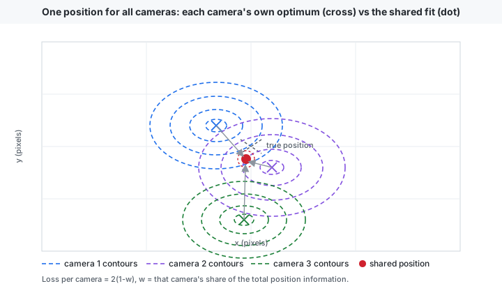
来源:公式与"一份 (1−w) 加真实数据的 m"读法见 reviews/T11_013_claude.md、reviews/T11_021_claude.md、reviews/T11_023_claude.md;模拟比值跨 Ŝ 分箱为 1.01–1.25(07 R013 放宽;早期读数 1.04–1.06 只是中心值,"与 S 无关"的措辞已撤回)。当前状态:2-D 位置损失本身 Provisional(量级对),"它单独闭合目录" Questioned,Q1 整体 open(闭合未证)——按模拟自己的口径目录是 −9.282 % [−9.350, −9.219](11,401 个观测;早先引用的 −10.4 % 不可复现,已撤回),15 幅图像的联合模拟试点用估计背景给到 A 臂 −5.9 %、B 臂 −7.4 %(差 3.39 % / 1.85 %),但试点与目录不匹配:b 0.028 恒定对 0.02→0.14,两个 6–10 窗口落在不同 \(\hat{S}\)(7.3–8.5 对 9.5–13),匹配 \(\hat{S}\) 后差 4–6 %,试点的亏损到 \(\hat{S}\) > 30 消失而目录停在 −7 %,试点 L2d/μ 5.0 % 对目录 9.8 %(07 R019;reviews/RT-26_triage_claude.md;此前读法见 07 R015)。图为示意,按公式重绘,非实测数据。Sources: the formula and the "one (1−w) plus the real-data m" reading are in reviews/T11_013_claude.md, reviews/T11_021_claude.md, reviews/T11_023_claude.md; the simulation ratio is 1.01–1.25 across Ŝ bins (widened by 07 R013; the early reading 1.04–1.06 is only the central value and its "independent of S" wording is withdrawn). Current status: the 2-D position loss itself is Provisional (right order); "it closes the catalogue alone" is Questioned, and Q1 as a whole is open (closure not shown) — under the simulation's own convention the catalogue is −9.282 % [−9.350, −9.219] (11,401 observations; the earlier −10.4 % is not reproducible and is withdrawn), and the 15-image joint-simulation pilot, scored with the estimated background, reaches arm A −5.9 % and arm B −7.4 % (gap 3.39 % / 1.85 %) but is not matched to the catalogue: b 0.028 flat against 0.02→0.14, the two 6–10 windows at different \(\hat{S}\) (7.3–8.5 against 9.5–13), 4–6 % at matched \(\hat{S}\), the pilot's deficit gone by \(\hat{S}\) > 30 while the catalogue stays at −7 %, and L2d/μ 5.0 % against 9.8 % (07 R019; reviews/RT-26_triage_claude.md; the earlier reading is 07 R015). The figure is illustrative, redrawn from the formula, not measured data.
算例:一台 MOS 相机在 15 幅图像里占 \(w = 1/15\),则 \(2(1-w) = 2 \times 14/15 \approx 1.87\)。若 μ + δ ≈ 20.5(第 4 节的算例),这一项就是约 9.1 % 的 ΔC——与目录在 6–10 的亏损同量级。剩下没被这一项解释的部分正是当前的主攻方向:按模拟自己的口径目录是 −9.282 % [−9.350, −9.219],联合模拟试点给到 −5.9 % / −7.4 % 但与目录不匹配(07 R019)。Worked example: one MOS camera is \(w = 1/15\) of 15 images, so \(2(1-w) = 2 \times 14/15 \approx 1.87\). With μ + δ ≈ 20.5 (the worked example in Section 4), that term is about 9.1 % of ΔC — the same order as the catalogue's 6–10 deficit. The part this term does not explain is the current focus: under the simulation's own convention the catalogue is −9.282 % [−9.350, −9.219], and the joint-simulation pilot reaches −5.9 % / −7.4 % but is unmatched to the catalogue (07 R019).
13. 小故事:拟合位置与宽度的关系——位置动的是均值,不是宽度13. A Short Story: The Fitted Position and the Width — The Position Moves the Mean, Not the Width
问题。理论给的宽度是 \(\sqrt{V(\hat{S})}\)。可实测里,拟合位置落在源附近的行和落在远处的行,\(\Delta C\) 的散布不一样。位置到底改变了什么?The question. The theory's width is \(\sqrt{V(\hat{S})}\). But in the data, rows whose fitted position lands near the source and rows whose fit lands far away have different \(\Delta C\) scatter. What does the position actually change?
先说人话。曾经的说法是:拟合位置落在源附近时位置误差被"压小",所以散布接近理论甚至略窄;被背景涨落吸到远处时位置误差突然变大,把亮度也拖歪,散布就宽。这个机制没有被证实,本段按 R055 / R059 改写。把行按可观测 \(\hat{S}\) 分箱后,在固定的窄 \(\hat{S}\) 上,宽度对拟合位置 \(\hat{r}\) 是平的——在 \(\hat{r} \leq\) 4 px 的核内,宽度并不随 \(\hat{r}\) 系统性变窄或变宽;动的是均值。真正让低 \(\hat{S}\) 处宽度偏窄的是另一件事:\(\hat{S}\) 小的时候,进入这个箱的行大多是真实流量向下涨落的那些,而给定 \(\hat{S}\) 的条件方差本身就小——这是一个低计数性质,不是位置被锁定的后果。至于远处那些行,它们不是"位置误差把宽度拖宽":它们在低 \(\hat{S}\) 箱里只占 13–26 %,却把全部行的 std 抬到 1.4–1.9,所以"全行宽度宽"是少数极端行的混合效应。位置当然重要——它决定均值往哪儿偏(\(\hat{r}\) 越大均值越偏),但它不是宽度的调节钮。Plain words first. The old story was: when the fitted position lands near the source the position error is "squeezed" small, so the scatter is close to theory or slightly narrow; when the fit is pulled onto a far background fluctuation the position error suddenly grows and drags the amplitude with it, so the scatter widens. That mechanism was not established and this paragraph is rewritten per R055 / R059. Binning the rows by the observable \(\hat{S}\), at fixed narrow \(\hat{S}\) the width is flat in the fitted position \(\hat{r}\) — inside the \(\hat{r} \leq\) 4 px core the width does not systematically narrow or widen with \(\hat{r}\); what moves is the mean. What actually narrows the width at low \(\hat{S}\) is something else: at small \(\hat{S}\) the rows entering that bin are mostly the downward fluctuations of the true flux, and the conditional variance given \(\hat{S}\) is itself small — a low-count property, not a consequence of the position being locked. As for the far rows, they are not "the position error widening the width": at low \(\hat{S}\) they are only 13–26 % of the rows, yet they lift the all-row std to 1.4–1.9, so "the all-row width is wide" is a mixture effect from a few extreme rows. The position matters, of course — it decides where the mean goes (the larger \(\hat{r}\), the more the mean shifts) — but it is not the width's dial.
怎么测的。两个口径,都只按可观测量(\(\hat{S}\)、b、拟合位置 \(\hat{r}\))分箱,从不按 ML 或 \(\Delta C\) 切行。(1) L0 生产表(我们自己的全局搜索拟合器):在典型 DET_ML 6–10 窗口内,把近行按 \(\hat{r}\) 细分,看未修正的 std z 怎么随 \(\hat{r}\) 走。(2) 玩具模拟(15\(\times\)15 高斯 PSF,位置自由):把行在一个 \(S_{true}\) 先验上汇成总体,再按可观测 \(\hat{S}\) 分箱,在固定 \(\hat{S}\) 上看宽度对 \(\hat{r}\) 的依赖。How it was measured. Two conventions, both binning only by observables (\(\hat{S}\), b, the fitted position \(\hat{r}\)), never cutting rows on ML or \(\Delta C\). (1) The L0 production table (our own global-search fitter): inside the typical DET_ML 6–10 window, sub-divide the near rows by \(\hat{r}\) and watch the uncorrected std z. (2) The toy simulation (15\(\times\)15 Gaussian PSF, position free): pool the rows into one population over an \(S_{true}\) prior, then bin by the observable \(\hat{S}\) and look at the width's dependence on \(\hat{r}\) at fixed \(\hat{S}\).
结果。左图(L0,未修正):近行里未修正的 std z 随 \(\hat{r}\) 先降后升——0.879(\(\hat{r}\) < 0.5 px)、0.863(0.5–1)、0.833(1–2),到 2–5 px 掉到 0.730,贴壁的行(\(\hat{r} \geq\) 10 px)又回到 0.917。注意:这个最小值在 \(\hat{r}\) 2–5 px,不是"越靠近源越窄"的单调趋势;按 R055 / R059,固定窄 \(\hat{S}\) 时宽度在 \(\hat{r}\) 上是平的,所以左图的形状主要是 \(\hat{r}\) 与 \(\hat{S}\) 的相关造成的,不能读成"拟合锁定源就让宽度变窄"。右图(玩具,可观测 \(\hat{S}\) 箱):核 r̂ \(\leq\) 4 px 的 std z 随典型 DET_ML 回到 1——1.3 时 0.822 \(\pm\) 0.006、3.0 时 0.889 \(\pm\) 0.007、4.8 时 0.929 \(\pm\) 0.007、7.4 时 0.964 \(\pm\) 0.007、11.8 时 0.993 \(\pm\) 0.007、26.8 时 0.997 \(\pm\) 0.007(b = 0.08;另一支独立人口 N = 12,000 全部在 1.4 SE 内一致)。The result. Left panel (L0, uncorrected): inside the near rows the uncorrected std z first falls and then rises with \(\hat{r}\) — 0.879 (\(\hat{r}\) < 0.5 px), 0.863 (0.5–1), 0.833 (1–2), falling to 0.730 at 2–5 px, with the wall-hugging rows (\(\hat{r} \geq\) 10 px) back at 0.917. Note: the minimum sits at \(\hat{r}\) 2–5 px, not on a monotone "the nearer the source, the narrower" trend; per R055 / R059 the width is flat in \(\hat{r}\) at fixed narrow \(\hat{S}\), so the left panel's shape is mostly the \(\hat{r}\)–\(\hat{S}\) correlation and must not be read as "the fit locking onto the source narrows the width". Right panel (toy, observable \(\hat{S}\) bins): the core r̂ \(\leq\) 4 px std z returns to 1 with typical DET_ML — 0.822 \(\pm\) 0.006 at 1.3, 0.889 \(\pm\) 0.007 at 3.0, 0.929 \(\pm\) 0.007 at 4.8, 0.964 \(\pm\) 0.007 at 7.4, 0.993 \(\pm\) 0.007 at 11.8 and 0.997 \(\pm\) 0.007 at 26.8 (b = 0.08; an independent population with N = 12,000 agrees within 1.4 SE in every bin).
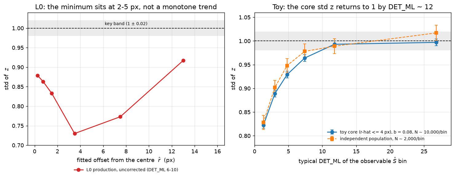
来源:左图数字逐字引自 E171 修正(07 R052,W3 Hermes 臂;与 RT-50 的 R050 趋势一致)——但左图的形状按 R055 / R059 重新解释,不再读作位置锁定。右图逐字引自 reviews/RT-55_triage_claude.md 的复算表(07 R059,T233 Provisional)与 03_TRUST_TABLE.md 的 T233 行。本页只作图、未重算。Source: the left panel's numbers are quoted verbatim from the E171 amendment (07 R052, the W3 Hermes arm; consistent with RT-50's R050 trend) — but the left panel's shape is reinterpreted per R055 / R059 and is no longer read as position locking. The right panel is quoted verbatim from the replay table in reviews/RT-55_triage_claude.md (07 R059, T233 Provisional) and the T233 row of 03_TRUST_TABLE.md. This page only draws them; nothing was recomputed.
14. 小故事:为什么按"真实流量"分箱会把偏窄放错位置14. A Short Story: Why Binning by the TRUE Flux Puts the Narrowing in the Wrong Place
问题。玩具模拟里,"插入式宽度在低 DET_ML 偏窄"曾经是在固定真实流量 \(S_{true}\) 的格子里量的:每个格子只放一批真实流量相同的源,再看格内 \(\hat{S}\) 最低的那个四分位。这样量出来,偏窄被定位在"每个格子里 \(\hat{S}\) 最低的那批源"上,还带着一句"DET_ML 8–14 窄 2–4 %"。可是翻目录的人并不知道 \(S_{true}\)——他只有 \(\hat{S}\)。同一个偏窄,换成只有目录里那些数也能做的分箱,还在老地方吗?The question. In the toy simulation, "the plug-in width is narrow at low DET_ML" was once measured inside fixed-\(S_{true}\) cells: each cell held one batch of sources with the same true flux, and then one looked at the lowest \(\hat{S}\) quartile inside the cell. Measured that way, the narrowing was located on "the lowest-\(\hat{S}\) sources inside each cell", together with the sentence "narrow by 2–4 % at DET_ML 8–14". But someone reading the catalogue does not know \(S_{true}\) — they only have \(\hat{S}\). Does the same narrowing stay in the old place when the binning is redone with only the numbers a catalogue reader has?
先说人话。固定 \(S_{true}\) 的格子是一个"上帝视角"的分箱:它按源本来有多亮来分组。可在一个格子里,源的亮度还是会上下涨落,而 \(\hat{S}\) 最低的那四分位,装的就是这批源里向下涨落的那些。于是"低 \(\hat{S}\)"在这个口径里同时意味着两件事:真实流量不算太低(格子定的),但这一回运气不好、量出来的偏暗。而给定 \(\hat{S}\) 的条件方差,本来在 \(\hat{S}\) 小的时候就小——所以偏窄当然出现在那里。这不是一条关于可观测量的律,这是分箱方式自己造出来的位置。换成目录读者能做的分箱(把行按一个 \(S_{true}\) 先验汇成一个总体,再按可观测 \(\hat{S}\) 分箱),偏窄还在,但它的位置和大小都变了:它整整齐齐地跟着 \(\hat{S}\)(也就是 DET_ML)走,在 DET_ML 1–3 最大,到 DET_ML \(\approx\) 12 就回到 1。Plain words first. A fixed-\(S_{true}\) cell is a "God's-eye" binning: it groups sources by how bright they really are. But inside one cell the brightness still fluctuates, and the lowest \(\hat{S}\) quartile holds exactly those rows of the batch that fluctuated downward. So "low \(\hat{S}\)" in that convention means two things at once: the true flux is not too low (the cell fixed it), but this particular draw was unlucky and measured faint. And the conditional variance given \(\hat{S}\) is itself small when \(\hat{S}\) is small — so of course the narrowing shows up there. That is not a law of the observables; it is a position created by the binning itself. Redoing it with the binning a catalogue reader can do (pool the rows into one population over an \(S_{true}\) prior, then bin by the observable \(\hat{S}\)), the narrowing is still there, but both its place and its size change: it follows \(\hat{S}\) (hence DET_ML) cleanly, is largest at DET_ML 1–3 and is back to 1 by DET_ML \(\approx\) 12.
怎么测的。两个口径都用同一批玩具行(15\(\times\)15 高斯 PSF,位置自由,项目拟合器,两个起点),都只按可观测量分箱,从不按 ML 或 \(\Delta C\) 切行。(1) 固定 \(S_{true}\) 格子(老口径):每个 \((b, S_{true})\) 格子内取 \(\hat{S}\) 的四分位。在 \((0.02, 6.63)\) 这个格子里,四个四分位的 std z 是 0.883 / 0.974 / 0.984 / 1.000;在 \((0.08, 10.80)\) 是 0.901 / 0.963 / 0.960 / 1.005。偏窄 12 % 在最低四分位,往上迅速消失。(2) 可观测 \(\hat{S}\) 箱(新口径,R059):把行按 dN/dS \(\propto S^{-2.5}\) 的先验汇成总体(b = 0.02 保留 58,986 行,b = 0.08 保留 59,810 行),再按 \(\hat{S}\) 等数分 6 箱,只统计核 r̂ \(\leq\) 4 px 的行。How it was measured. Both conventions use the same toy rows (15\(\times\)15 Gaussian PSF, position free, the project fitter, two starts) and bin only by observables, never cutting rows on ML or \(\Delta C\). (1) Fixed-\(S_{true}\) cells (the old convention): take \(\hat{S}\) quartiles inside each \((b, S_{true})\) cell. In the \((0.02, 6.63)\) cell the four quartiles give std z 0.883 / 0.974 / 0.984 / 1.000; in \((0.08, 10.80)\), 0.901 / 0.963 / 0.960 / 1.005. The narrowing is 12 % in the lowest quartile and gone above it. (2) Observable \(\hat{S}\) bins (the new convention, R059): pool the rows into one population over a dN/dS \(\propto S^{-2.5}\) prior (58,986 rows kept at b = 0.02 and 59,810 at b = 0.08), then split into 6 equal-count \(\hat{S}\) bins and score only the core r̂ \(\leq\) 4 px rows.
结果。固定 \(S_{true}\) 格子的读数把偏窄说成"DET_ML 8–14 窄 2–4 %";可观测 \(\hat{S}\) 箱给出的是一条随 DET_ML 总体回到 1 的曲线(b = 0.02 在 4.9 是 0.953、7.5 是 0.944,并非严格单调),而且低端比老说法深得多:b = 0.02 是 0.860(典型 DET_ML 1.4)、0.846(3.0)、0.953(4.9)、0.944(7.5)、0.993(11.9)、1.003(26.7);b = 0.08 是 0.822(1.3)、0.889(3.0)、0.929(4.8)、0.964(7.4)、0.993(11.8)、0.997(26.8)。每个箱的 SE 都是 0.006–0.007,所以前四个箱离 1 有 5–28 个 SE,最后两个箱在 1 SE 内。也就是说:偏窄在 DET_ML 1–3 是 14–18 %(0.82–0.86,T233),在 \(\approx\) 5 是 5–7 %、\(\approx\) 7.5 是 4–6 %,到 DET_ML \(\approx\) 12 就没有了。老口径的"8–14 窄 2–4 %"其实是固定 \(S_{true}\) 格子里 \(\hat{S}\) 分布的低端尾巴造成的格子混合值。还有两件事老口径没报:均值也失效——最低箱的 mean z 是 +0.290(b = 0.02)与 +0.304(b = 0.08),离 0 有 30 个 SE(这两个均值只对 −2.5 源计数先验成立;宽度与先验无关,见 R063);全行宽度反而宽——最低箱把 r̂ \(\geq\) 4 px 的行算进来,std 是 1.44–1.89,因为那些行占 13–26 % 而 std 高达 1.3–7.5。The result. The fixed-\(S_{true}\) reading described the narrowing as "narrow by 2–4 % at DET_ML 8–14"; the observable \(\hat{S}\) bins give a curve that returns to 1 overall with DET_ML (b = 0.02 is 0.953 at 4.9 and 0.944 at 7.5, so it is not strictly monotone), and at the low end it is far deeper than the old wording: b = 0.02 gives 0.860 (typical DET_ML 1.4), 0.846 (3.0), 0.953 (4.9), 0.944 (7.5), 0.993 (11.9) and 1.003 (26.7); b = 0.08 gives 0.822 (1.3), 0.889 (3.0), 0.929 (4.8), 0.964 (7.4), 0.993 (11.8) and 0.997 (26.8). Every bin's SE is 0.006–0.007, so the first four bins are 5–28 SE from 1 and the last two are within 1 SE. That is: the narrowing is 14–18 % at DET_ML 1–3 (0.82–0.86, T233), 5–7 % at \(\approx\) 5 and 4–6 % at \(\approx\) 7.5, and gone by DET_ML \(\approx\) 12. The old convention's "2–4 % at 8–14" was really a cell-mix value produced by the low tail of the \(\hat{S}\) distribution inside the fixed-\(S_{true}\) cells. Two more things the old convention did not report: the mean fails too — the lowest bin's mean z is +0.290 (b = 0.02) and +0.304 (b = 0.08), 30 SE from 0 (these means hold only for the −2.5 source-count prior; the width is prior-independent, see R063); and the all-row width is wide instead — including the r̂ \(\geq\) 4 px rows, the lowest bin's std is 1.44–1.89, because those rows are 13–26 % of the bin with std as high as 1.3–7.5.
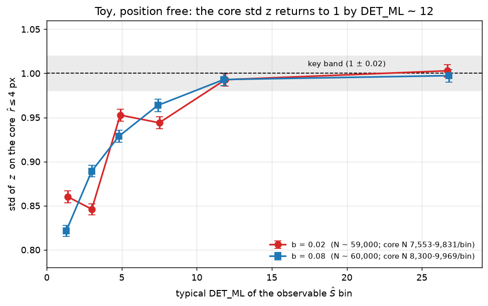
来源:07 R059(T233 改写为可观测律);固定 \(S_{true}\) 四分位数字逐字引自 RT-55 报告的 O1(复现在 codexnim 行上),可观测箱数字逐字引自同一报告的 O8 全量运行表(N \(\approx\) 59,000 每 b,virgo,种子 20261018 / 20261019);分诊见 reviews/RT-55_triage_claude.md。图为按引用数字重绘,未重算。Sources: 07 R059 (T233 rewritten as an observable law); the fixed-\(S_{true}\) quartile numbers are quoted verbatim from section O1 of the RT-55 report (reproduced on the codexnim rows) and the observable-bin numbers from the same report's O8 full-run table (N \(\approx\) 59,000 per b, on virgo, seeds 20261018 / 20261019); the triage is reviews/RT-55_triage_claude.md. The figure is redrawn from the quoted numbers; nothing was recomputed.
15. 真实 PSF 表现得像玩具吗?15. Does the Real PSF Behave Like the Toy?
玩具的可观测偏窄到 DET_ML \(\approx\) 12 就消失了。真实 PSF 的没有——它一直持续到目录区间。这条差别是 R062 带来的新事实,也是 Q7 现在剩下的最后一块。The toy's observable narrowing is gone by DET_ML \(\approx\) 12. The real PSF's is not — it lasts into the catalogue regime. That difference is the new fact R062 brought, and it is the last remaining piece of Q7.
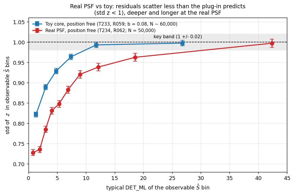
两条曲线在匹配的 DET_ML 上差得最多的地方是 DET_ML 5–20:DET_ML \(\approx\) 12 处玩具是 0.993(07 R059),真实 PSF 是 0.938(07 R062)。低端真实 PSF 也更深:0.73(DET_ML 0.75)对玩具的 0.82(1.3)。所以玩具的低端描述不能直接搬到真实 PSF 上。Matched in DET_ML, the two curves differ most at DET_ML 5-20: at DET_ML \(\approx\) 12 the toy is 0.993 (07 R059) and the real PSF 0.938 (07 R062). The real PSF is also deeper at the low end: 0.73 (DET_ML 0.75) against the toy's 0.82 (1.3). The toy's low-end description therefore cannot be carried over to the real PSF directly.
为什么均值要源计数先验,宽度不要(R063)。固定 \(\hat{S}\) 时,一个箱里混着的真实流量有哪些,取决于天上暗源多还是亮源多——这就是源计数先验 dN/dS。均值把这混合比例一起统计进去,所以它随先验移动(DET_ML \(\lesssim\) 17 以下);宽度是散布,混合比例怎么变它都只反映同一个源的散度,所以它与先验无关(建议(未经评审):这句解释不在任何记录里,R063 只记录了宽度在先验变化下移动不超过 0.036 这个实测结果)。Why the mean needs the source-count prior and the width does not (R063). At fixed \(\hat{S}\), which true fluxes are mixed into a bin depends on whether the sky has more faint or more bright sources — that is the source-count prior dN/dS. The mean averages over that mixing ratio, so it moves with the prior (below DET_ML \(\lesssim\) 17); the width is a spread, and it reflects the divergence of a single source however the mixing ratio changes, so it is prior-independent (Suggestion (not reviewed): this explanation is in no record; R063 records only the measured result that the width moves by at most 0.036 when the prior changes).
机制:两个几乎相消的大项,把 1 % 的错配放大成 8–16 % 的方差高估(R077/R078 定位,R086 统一两条流水线)。把 \(V_{3p}\) 展开成两项:\(V_{3p} = \mathrm{term1} - 4\,\mathrm{penalty}\)。这两项几乎完全相消——term1 是 Var(R) 的 15–31 倍,方差只来自两者之差。一个算例(RT-72,已复算):在 DET_ML \(\approx\) 3.5 这一箱,term1 = 63.6 而 Var(R) = 1.90(约 33 倍),penalty 错配 \(\approx\) 1.4 %,于是 \(V_{3p}(\hat{S})\)/Var(R) = 1.44——1 % 的一级误差变成约 44 % 的方差误差。错配随 PSF 的翼结构(低计数翼像素)与计数上升:同二阶矩的高斯只有 \(\approx\) 0.05 %,真实 PSF 是 +1.0–1.8 %;固定 \(\hat{S}\) 把 b 减半会把错配抬高 +0.5…+0.9 pp(\(\hat{S} \lesssim\) 5)。同一个机制也解释 emldetect(L1)的宽度(R086,RT-81,已复算):用合并估计量,L1 的 Fisher penalty 错配在 DET_ML 6–10 是 +1.19 % [+1.03, +1.35],解释了箱内 L1 宽度缺口的 0.89 [0.84, 0.93](预测 std z 0.919,实测 0.918;按行合并 0.940);错配随计数下降(+0.63 % 于 10–20,100 以上约 0)。R083 的 −0.14 % 是逐格比值的平均,已被 R086 推翻。
没有解析修正能闭合它:Bartlett 的 +2\(\cdot\)rank 项符号反了,beyond-Fisher 的位置曲率项过度修正 1.3–7.4 倍、在最低 \(\hat{S}\) 处给负方差、在最高分箱处变号(R080);按实测 MLE 偏差校准的振幅修正仍留 std z 0.952 / 0.959 / 0.968 / 0.972(R072),带 Fisher 展布的 \(E[V_{3p} \mid \hat{S}]\) 更差(0.84–0.96)。白话:两个几乎相等的大数相减,其中一个差 1 %,结果就差出 5–16 %——这就是残差看起来窄的原因,而且 PSF 越集中越明显。The mechanism: two nearly cancelling large terms amplify a 1 % mismatch into an 8–16 % variance over-statement (located by R077/R078, unified across both pipelines by R086). Expand \(V_{3p}\) into two terms: \(V_{3p} = \mathrm{term1} - 4\,\mathrm{penalty}\). The two nearly cancel — term1 is 15–31\(\times\) Var(R), and the variance is only the difference of the two. A worked example (RT-72, replayed): in the DET_ML \(\approx\) 3.5 bin, term1 = 63.6 against Var(R) = 1.90 (about 33\(\times\)) and the penalty mismatch is \(\approx\) 1.4 %, so \(V_{3p}(\hat{S})\)/Var(R) = 1.44 — a 1 % first-order error becomes about a 44 % variance error. The mismatch rises with the PSF's wing structure (low-count wing pixels) and the counts: a Gaussian of equal second moment has only \(\approx\) 0.05 % while the real PSF has +1.0–1.8 %; halving b at fixed \(\hat{S}\) raises the mismatch by +0.5…+0.9 pp (\(\hat{S} \lesssim\) 5). The same mechanism explains emldetect's (L1) width too (R086, RT-81, replayed): with pooled estimators the L1 Fisher-penalty mismatch at DET_ML 6–10 is +1.19 % [+1.03, +1.35], explaining 0.89 [0.84, 0.93] of the within-cell L1 width deficit (predicted std z 0.919, observed 0.918; row-pooled 0.940); the mismatch falls with counts (+0.63 % at 10–20, about 0 above 100). R083's −0.14 % was a mean of per-cell ratios and is reversed by R086.
No analytic correction closes it: the Bartlett +2\(\cdot\)rank term has the wrong sign, and the beyond-Fisher position-curvature term over-corrects by 1.3–7.4\(\times\), gives a negative variance at the lowest \(\hat{S}\) and flips sign at the top bin (R080); an amplitude correction calibrated to the measured maximum-likelihood bias still leaves std z 0.952 / 0.959 / 0.968 / 0.972 (R072), and \(E[V_{3p} \mid \hat{S}]\) with a Fisher spread is worse (0.84–0.96). In plain words: two nearly equal large numbers are subtracted, one of them is off by 1 %, and the result is off by 5–16 % — that is why the residual looks narrow, and the more concentrated the PSF the worse it gets.
白话:低计数端的中心项偏高是 L0 这条流水线自己的性质,不是 emldetect 的物理(R082、R084、R085;成因 R087 之后开放)。把 L0 的同一批 stamp 用一个匹配对照重放——同样的 PSF 栅格、同样的掩膜、同样的背景律、同样的抖动、同一个位置——差距就不再是“物理”,而是“L0 这条流水线怎么把光加起来”。用 L0 自己的 \(S_{true}\) 支撑重建对照(4 个种子)后,按可观测 \(\hat{S}\) 分箱的差距是:\(\hat{S}\) < 4 处 +0.389,\(\hat{S}\) 4–11 处 +0.18/+0.15/+0.15/+0.15/+0.15/+0.14,\(\hat{S}\) \(\geq\) 11 处 +0.058 \(\pm\) 0.007(原写的 +0.148 是对照支撑被截断造成的),到高计数锚(DET_ML 典型值 \(\geq\) 50)处 −0.006 \(\pm\) 0.020,两侧都约 0。归因已撤回(R087,RT-83,已复算):把同一批匹配对照图用 FFT 模板族与 v2t1 重新拟合(配对,10,000 行),中心位移在 \(\hat{S}\) < 4 处为 −0.003(精确 plug-in)或 +0.037 \(\pm\) 0.034(核 \(\delta\)),只补上 0–27 % 的差距,不是 72 %;超额本身(上表)仍然成立,其成因开放。同一机制也解释 L1(emldetect)的宽度(R086,RT-81,已复算):用合并估计量,L1 的 Fisher penalty 错配在 DET_ML 6–10 是 +1.19 % [+1.03, +1.35],解释了箱内 L1 宽度缺口的 0.89 [0.84, 0.93](预测 std z 0.919,实测 0.918;按行合并 0.940)。R083 的 −0.14 % 是逐格比值的平均,已被 R086 推翻;“BG_MAP_EML 是原因”也被驳回(它就是图像自己的背景)。所以同一个 \(V_{3p}\) 机制同时决定 L0 与 emldetect 的宽度(配对实验 0b 已完成:R089)。
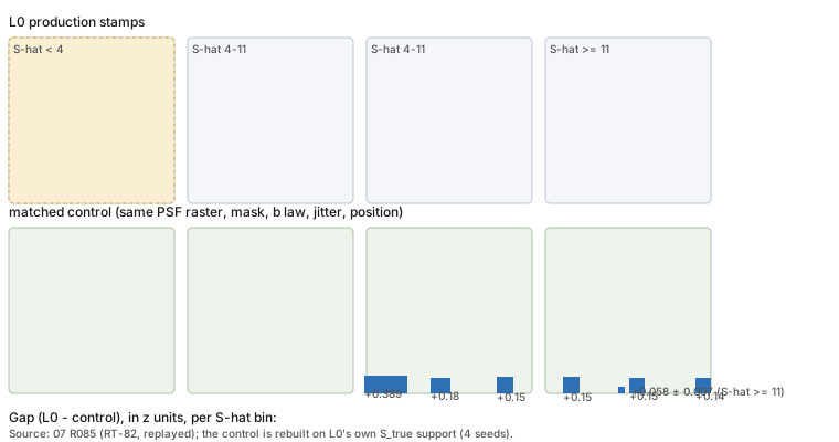
来源:07 R085(RT-82,已复算);对照在 L0 自己的 \(S_{true}\) 支撑上用 4 个种子重建。Source: 07 R085 (RT-82, replayed); the control was rebuilt on L0's own \(S_{true}\) support with 4 seeds.
In plain words: the low-count centre excess is a property of the L0 pipeline itself, not of emldetect physics (R082, R084, R085; its cause is open after R087). Replay the same L0 stamps with a matched control — the same PSF raster, the same mask, the same background law, the same jitter, the same position — and the gap stops being “physics” and becomes “how the L0 pipeline adds the light up”. With the control rebuilt on L0's own \(S_{true}\) support (4 seeds), the gaps in observable \(\hat{S}\) bins are: +0.389 at \(\hat{S}\) < 4, +0.18/+0.15/+0.15/+0.15/+0.15/+0.14 at \(\hat{S}\) 4–11, +0.058 \(\pm\) 0.007 at \(\hat{S}\) \(\geq\) 11 (the earlier +0.148 came from truncated control support), and −0.006 \(\pm\) 0.020 at the high-count anchor (DET_ML-typical \(\geq\) 50), about 0 on both sides. The attribution is withdrawn (R087, RT-83, replayed): refitting the same matched-control images with the FFT family and v2t1 (paired, 10,000 rows) shifts the centre by −0.003 (the exact plug-in) or +0.037 \(\pm\) 0.034 (the kernel \(\delta\)) at \(\hat{S}\) < 4, closing only 0–27 % of the gap, not 72 %; the excess itself (the table above) still stands, and its cause is open. The same mechanism does explain the L1 (emldetect) width (R086, RT-81, replayed): with pooled estimators the L1 Fisher-penalty mismatch at DET_ML 6–10 is +1.19 % [+1.03, +1.35], explaining 0.89 [0.84, 0.93] of the within-cell L1 width deficit (predicted std z 0.919, observed 0.918; row-pooled 0.940). R083's −0.14 % was a mean of per-cell ratios and is reversed by R086; the “BG_MAP_EML is the cause” reading is rejected (it is the image's own background). So the same \(V_{3p}\) mechanism carries both the L0 and the emldetect widths (the paired experiment 0b is completed: R089).
这条规律不止在一个位置,也不止一条流水线(R065/R066/R067,RT-62/61/64 分诊;R086 统一)。在 L0 生产数据的全部 67 个位置(离轴 0–13′)上它都成立,数值比单一位置低约 0.02:合并 std z 0.840 / 0.894 / 0.909 / 0.959 / 0.984 于 DET_ML \(\approx\) 4.6 / 7.9 / 11.1 / 22.8 / 36.8,到 DET_ML \(\approx\) 36–60 才回到 1。L1(emldetect)的低端偏窄比 L0 浅得多(std z 0.94–0.98 于 DET_ML 1–6、\(\approx\) 0.95 于 6–10、12–20 以上约 1,最低一箱反而宽 1.31)。R086 之后这个差有了归宿:同一个 \(V_{3p}\) 相消机制在两条流水线上都起作用,L1 的错配较小(+1.19 % 对 L0 的 +1.0–1.8 %),所以它的偏窄也较浅——量的差别,不是物理的差别。剩余的差(匹配比较下 L1 − L0 = +0.24 / +0.19 / +0.12 / +0.08 / +0.07 于 DET_ML \(\approx\) 2–7)来自两边不同的打分与振幅估计量(真实 PSF 模板族在拟合位置 对 替代核在名义位置;\(E[\hat{S}]/E[S_{eml}]\) = 1.38 于 \(S_{true}\) 2.5)。白话:机制统一了,剩下的问题是“拟合器在上面加了多少”。任务 0b(同图同打分的配对实验,只让拟合器不同)已完成(R089,已复算):同一批 bit-exact L0 图像上,emldetect 与 L0 在高计数锚一致(模型典型 DET_ML ≥ 50:L0 −0.008/0.978,emldetect −0.012/0.971;Ŝ ≳ 19 处 Δmean、Δstd 在 ±0.02 内),DET_ML ≲ 7 处 emldetect 中心比 L0 低 0.16–0.53 z、宽 0.05–0.14(3 个试点位置;最低 Ŝ 箱 N_eff 6–55)。所以 L0 的低计数中心项超额不是 emldetect 的性质,单图 emldetect 规律必须在 emldetect 输出(L1/0b)上建立,不能从 L0 搬用。规律阶段(R093–R104,2026-10-21 被一次专家复核改写):宽度的一半在"同一个位置内"解决了,中心的一半还开着,而且两个目标必须分开说。在 emldetect 输出(M2 能段 4)上,PI 主线规律 \(p(\mathrm{DET\_ML} \mid \hat{S}, b, \mathrm{index})\) 的四个候选依次被检验:插入式 C 10/72、制表修正 D 48/72、二次 index 的 DQ 42/72、生成式混合 MIX3d 35/72(留出格通过数;一支在"恰好为真"数据上验证过的评分器把四条全部拒收,零假设均值约 62–63/72,D 的 p = 0.0015)。这些通过数自此是历史诊断,不是当前得分(R118 取代)。原因是打分手本身混用了三个不同的估计对象(R114,专家复核,已采纳):宽度是每个位置各自减去自己的加权均值之后的 std("位置内"宽度),均值与覆盖率却把各位置的行合并起来算,而零假设的位置散布还是从候选自己的留出残差估的。RT-98(R117,已复算)把这一点做到了精确:位置内的二阶矩对任何常数位置偏移恒等不变(1e-15)——一条位置内校准精确、但带 0.30 z 逐位置偏移的规律,仍然通过宽度 70/72,而 cov68 的失败从 4 涨到 29。所以"宽度可以推广"这句话只能读作"在同一个位置内成立"。新的打分手(SCORER-CONTRACT v2,R118,已复算)把两个目标分开:未见位置总体上 D / H2 / MIX3d / C 通过 44 / 50 / 32 / 12 格(共 72,能段 4),能段 1 的 D / H2 为 36 / 43,全部被 Q 拒(p \(\leq\) 0.009);R124 限定:这是一次不稳定的抽样——14 个位置分半上 D 22–46、H2 26–52(能段 4),能段 1 的 D 14–53、H2 30–52;H2 优于 D 在固定分半上不显著(McNemar p 0.18 / 0.25),所以不能作"H2 最好"的排名,任何规律排名之前先要 scorer v3;逐位置上每条规律都大幅失败(能段 4 为 1 / 0 / 1 / 0,能段 1 为 0 / 1),冻结的位置效应 \(\tau_{mean}\) 是 0.14 z(能段 4)与 0.18 z(能段 1),重尾(df \(\approx\) 3)——位置效应本身比 0.05 的均值容差大,所以逐位置目标不能靠合并格通过。中心项的主导成分是 D 表自身的样本内表征误差(R116:把同一个位置内新的独立重复拿来打分,失败 24 \(\to\) 3;拿到未见位置上 21 \(\to\) 8,用的是 72 参数的逐格诊断修正),不是位置泛化缺口;专家那条先验混合恒等式作为代数成立(闭合到 1e-9),但它的协方差项在失败格里比观测误差大 2–8 倍、且已被 D 自己拟合的 \(\beta\) 斜率抵消(RT-99),所以它不是那个未解决的残差。宽度项的读数也被限定(R115):那个 0.976 [0.956, 0.993] 的留出宽度只是一次偏低的分半,40 个按半径分层的分半平均是 0.998;6 参数修正只通过 25/72 个宽度格。位置也不是缺失的变量:平滑的离轴/PSF 项把留出失败从 24 个推到 58–72 个(CENTRE-POS),负均值 z 是逐格(计数箱)中心偏置。所以"已解决"的只是宽度在同一个位置内的那一半(机制统一,R086),仍开放的是中心项(负、中计数、随 index 增长)与它对单个拟合位置的依赖(R104)。白话:宽度知道为什么错了——但"对"是在一个位置内对的;中心还不知道,而且现在知道它大部分是表格自己没拟合好,不是位置搬不动。The law is not a one-position artefact, and after R086 it is not a one-pipeline artefact either (R065/R066/R067, the RT-62/61/64 triages; unified by R086). It holds at all 67 L0 production positions (off-axis 0–13 arcmin), about 0.02 below the single position: pooled std z 0.840 / 0.894 / 0.909 / 0.959 / 0.984 at DET_ML \(\approx\) 4.6 / 7.9 / 11.1 / 22.8 / 36.8, reaching 1 only at DET_ML \(\approx\) 36–60. L1 (emldetect) shows a much shallower low-end narrowing (std z 0.94–0.98 at DET_ML 1–6, \(\approx\) 0.95 at 6–10, about 1 above 12–20, the lowest bin wide at 1.31). After R086 this difference has a home: the same \(V_{3p}\) cancellation mechanism acts in both pipelines, and L1's mismatch is smaller (+1.19 % against L0's +1.0–1.8 %), so its narrowing is shallower too — a difference of degree, not of physics. The remaining gap (in the matched comparison L1 − L0 = +0.24 / +0.19 / +0.12 / +0.08 / +0.07 at DET_ML \(\approx\) 2–7) comes from the two sides' different scoring and amplitude estimands (the real-PSF template family at the fitted offset against a surrogate kernel at the nominal position; \(E[\hat{S}]/E[S_{eml}]\) = 1.38 at \(S_{true}\) 2.5). In plain words: the mechanism is unified; what remains to measure is “how much the fitter adds on top”. Task 0b (the paired same-images same-scoring run, so that only the fitter differs) is completed (R089, replayed): on the same bit-exact L0 images emldetect and L0 agree at the high-count anchor (model-typical DET_ML ≥ 50: L0 −0.008/0.978, emldetect −0.012/0.971; at Ŝ ≳ 19 Δmean and Δstd within ±0.02) and at DET_ML ≲ 7 emldetect's centre is 0.16–0.53 z lower and its width 0.05–0.14 larger than L0 (3 pilot positions; lowest-Ŝ bins N_eff 6–55). So the L0 low-count centre excess is not an emldetect property, and the single-image emldetect law must be measured on emldetect output (L1/0b), not taken from L0.The law stage (R093–R104, rewritten on 2026-10-21 by an expert review): the width half is solved "within one position"; the centre half is still open, and the two targets must be stated separately. On emldetect output (M2 band 4), the PI main-line law \(p(\mathrm{DET\_ML} \mid \hat{S}, b, \mathrm{index})\) had four candidates tested in turn: the plug-in C 10/72, the tabulated correction D 48/72, the quadratic-index DQ 42/72 and the generative mixture MIX3d 35/72 (held-out cell passes; one scorer validated on exactly-true data rejects all four, null mean about 62–63/72, D's p = 0.0015). Those pass counts are historical diagnostics from here on, not the current score (superseded by R118). The reason is that the scorer itself mixed three different estimands (R114, the expert review, accepted): the width is the std after each position subtracts its own weighted mean (a "within-position" width), the mean and coverage pool rows across positions, and the null's position scatter is estimated from the candidate's own held residuals. RT-98 (R117, replayed) made this exact: the within-position second moment is identically invariant (1e-15) to any constant per-position offset — a law with exact within-position calibration but a 0.30 z per-position offset still passes width 70/72, while cov68 failures rise from 4 to 29. So "the width generalises" can only be read as "within one position". The new scorer (SCORER-CONTRACT v2, R118, replayed) separates two targets: on the population of unseen positions D / H2 / MIX3d / C pass 44 / 50 / 32 / 12 of 72 cells (band 4) and band-1 D / H2 36 / 43, all rejected on Q (p \(\leq\) 0.009); R124 qualifies: these are one draw of an unstable statistic — over 14 position splits D 22–46 and H2 26–52 (band 4), band-1 D 14–53 and H2 30–52; H2 above D is not significant on the fixed split (McNemar p 0.18 / 0.25), so no "H2 is best" ranking can be made, and scorer v3 is needed before any law ranking; per position every law fails by a wide margin (band 4: 1 / 0 / 1 / 0; band 1: 0 / 1), with the frozen position effect \(\tau_{mean}\) 0.14 z (band 4) and 0.18 z (band 1), heavy-tailed (df \(\approx\) 3) — the position effect itself is larger than the 0.05 mean tolerance, so the per-position target cannot be met by passing pooled cells. The centre term is dominated by an in-sample representation error of the D table itself (R116: scoring new independent realisations at the same positions takes the failures 24 \(\to\) 3, and at unseen positions 21 \(\to\) 8 with a 72-parameter per-cell diagnostic correction), not a position-generalisation gap; the expert's prior-mixing identity holds as algebra (closing to 1e-9), but its covariance term is 2–8\(\times\) the observed error in the failing cells and is already cancelled by D's own fitted \(\beta\) slope (RT-99), so it is not the unresolved residual. The width term's reading is qualified too (R115): that 0.976 [0.956, 0.993] held-out width was one low split, and the average over 40 radius-stratified splits is 0.998; the 6-parameter correction passes only 25/72 width cells. Position is not the missing variable either: a smooth off-axis/PSF term pushes the held-out failures from 24 to 58–72 (CENTRE-POS), so the negative mean z is a per-cell (count-bin) centre bias. What is solved is therefore only the width half within one position (the mechanism is unified, R086); what is open is the centre term (negative, mid-count, growing with index) and its dependence on one fitted position (R104). In plain words: for the width we know why it is wrong — but "right" is right within one position; for the centre we do not yet know, and we now know most of it is the table failing to fit itself, not the position being un-transferable.
来源:07 R062、R063、R064、R065、R066、R067、R068、R069、R070、R071、R072、R074、R075、R076、R077、R078、R080;真实 PSF 分箱数字逐字引自 RT-58 的分诊与其报告 §2,校准偏差与噪声凸性算例逐字引自 reviews/RT-67_triage_claude.md 的复算表,玩具核数字逐字引自 §14 的 T233 表,凸性与 +14.5 % / 1.6 的算例数字逐字引自 reviews/RT-60_triage_claude.md 的复算表,67 位置数字引自 reviews/RT-62_triage_claude.md,L1 与匹配比较引自 reviews/RT-61_triage_claude.md 与 reviews/RT-64_triage_claude.md,偏差校正修正的推翻引自 reviews/RT-63_triage_claude.md。图为按引用数字重绘,未重算。口径错误的短故事逐字引自 07 R158、R162、R167 与 reviews/RT-117、RT-119 的复算(0.7273 vs 0.6061,两口径均逐位复现)。判据太脆的短故事逐字引自 07 R220、R229 与 reviews/RT-138 的复算(基线 4 个失败箱、−1/3 箱移 2 个、+1/3 箱移 4 个)。Sources: 07 R062, R063, R064, R065, R066, R067, R068, R069, R070, R071, R072, R074, R075, R076, R077, R078, R080; the real-PSF bin numbers are quoted verbatim from RT-58's triage and its report §2, the toy-core numbers verbatim from the T233 table in §14, the convexity and +14.5 % / 1.6 worked-example numbers verbatim from the replay table in reviews/RT-60_triage_claude.md, the 67-position numbers from reviews/RT-62_triage_claude.md, the L1 and matched-comparison numbers from reviews/RT-61_triage_claude.md and reviews/RT-64_triage_claude.md, the calibrated-bias and noise-convexity worked example verbatim from the replay table in reviews/RT-67_triage_claude.md, and the refutation of the bias-corrected correction from reviews/RT-63_triage_claude.md. The figure is redrawn from the quoted numbers, not recomputed. The convention-error short story is quoted verbatim from 07 R158, R162, R167 and the RT-117 / RT-119 replays (0.7273 vs 0.6061, both conventions reproduced bit-for-bit). The brittle-rule short story is quoted verbatim from 07 R220, R229 and the RT-138 replay (4 failing bins at baseline, 2 under a −1/3-bin shift, 4 under a +1/3-bin shift).
再说一遍宽度的账,因为它是"已解决"的那一半。在固定的模型下,\(\Delta C = D_{null} - D_{best}\) 的均值 \(\mu_{3p}\) 和方差 \(V_{3p}\) 都能从像素和精确算出来(Z 的 std 是 0.998)。为什么?因为逐像素看,\(d_{null} - d_{best} = 2[y \ln(\mu/b) - (\mu - b)]\) 里的 \(y \ln y\) 饱和项在两个模型相减时抵消了,所以 \(\Delta C\) 在模型固定时对数据是线性的——线性量的方差就是逐像素方差之和 \(V_{3p}\),没有高阶修正。难的地方在别处:真正要算的不是在真实参数处的 \(\Delta C\),而是在拟合出来的参数 \(\hat{\theta}\) 处的 \(\Delta C\)。它的均值已经解到二阶(E088 的 \(\delta_0\)、E090 的 \(\delta_1\),Bartlett 修正,跟 Li et al. 2025 arXiv:2510.03466 的定理 6 同一套展开),不带任何拟合系数——但只对理论匹配的拟合器成立(R123):在 emldetect 自己的统计量上 \(\delta_1\) 在 36/36 个格里高估均值偏移(+0.19…+0.85 \(\Delta C\),均值 +0.44),而 \(\delta_0\) 保持在 0.12 sd 内,所以对 emldetect 与论文只能引用 \(\delta_0\) 的均值结果。它的方差的类比量已由 WIDTH-2ND 推进到第一个闭式解,但预注册判据未过(R121,2026-10-21 14:16 EDT,PI 06:20 EDT 批准):宽度亏缺被重新归因为条件方差 \(\mathrm{Var}[\Delta C \mid \hat{\theta}] < V_{3p}(\hat{\theta})\)——箱内 \(S_{true}\) 混合可忽略且只会增大方差(0.000–0.014),条件均值项同样可忽略(0.000–0.010)。新的 \(O(n^{-1})\) 闭式因子 \(c = 1 - \mathrm{tr}(I^{-1}Q)/(2V_{3p}) - \mathrm{tr}(I^{-1}P)^2/(4V_{3p})\)(\(P = \sum r\,\mu_a\mu_b/\mu\),\(Q = \sum r^2\,\mu_a\mu_b/\mu\))与暴力 Edgeworth 展开吻合到小数点后四位;在 \(b = 0.01\) 处精确(对数误差均方根 3.1 %,DET_ML 6–20 的修正宽度在 1 的 1.6\(\sigma\) 内),但在 \(b = 0.04\) 欠修(0.952 \(\pm\) 0.013,−3.6\(\sigma\))、\(b = 0.16\) 更差(0.926 \(\pm\) 0.012,−6.1\(\sigma\)),预注册判据 FAIL(8 个箱里 3 个超出 2\(\sigma\))。残差跟随 \(V_{3p}\) 的相消因子 \(4\sum\mu L^2/V_{3p}\)(\(R^2\) 0.89),不跟随 \(n_{\rm eff}\);猜想是高 \(b\) 处 \(L \approx (S/b)p\) 与 S-score 近平行,\(O(n^{-1})\) 展开在那里失效。白话:均值的高阶项有公式;方差的高阶项在低背景处也有了闭式解,但高背景处展开失效——下一步是沿 S-score 方向的重求和/精确条件方差。2026-10-22 更新:第一条可观测的箱级宽度规律 \(\bar{V}(\hat{S}, b) = E[V2 \mid \hat{S}, b]\)(拟合半、对 S 的后验)在 PI 批准的“8 箱允许 1 箱失败”判据下通过(R146;R152:带宽在测试半上选定,40 个随机分半平均 0.91 个失败箱,P(\(\leq\) 1) 0.79);构造迁到 emldetect 行成立,但全统计量下仍失败 5/5 箱(R151)——每个流水线要各自重建。The width ledger once more, because it is the "solved" half. At fixed models, the mean \(\mu_{3p}\) and variance \(V_{3p}\) of \(\Delta C = D_{null} - D_{best}\) both follow exactly from the pixel sum (the std of Z is 0.998). Why? Because pixel by pixel, the \(y \ln y\) saturation term in \(d_{null} - d_{best} = 2[y \ln(\mu/b) - (\mu - b)]\) cancels when the two models are subtracted, so \(\Delta C\) is linear in the data at fixed models — and the variance of a linear quantity is just the pixel sum \(V_{3p}\), with no higher-order correction. The hard part is elsewhere: what must actually be computed is not \(\Delta C\) at the true parameters, but \(\Delta C\) at the fitted parameters \(\hat{\theta}\). Its mean is solved to second order (E088's \(\delta_0\) and E090's \(\delta_1\), the Bartlett correction, the same expansion machinery as Li et al. 2025 arXiv:2510.03466's Theorem 6), with no fitted coefficient — but only for the theory-matched fitter (R123): on emldetect's own statistic \(\delta_1\) over-predicts the mean shift in 36 of 36 cells (+0.19…+0.85 \(\Delta C\), mean +0.44) while \(\delta_0\) stays within 0.12 sd, so for emldetect and the paper only the \(\delta_0\) mean result may be quoted. The variance analogue has reached a first closed form, but the pre-registered key is not met (R121, 2026-10-21 14:16 EDT; WIDTH-2ND was approved by the PI at 06:20 EDT): the width deficit is re-attributed to the conditional variance \(\mathrm{Var}[\Delta C \mid \hat{\theta}] < V_{3p}(\hat{\theta})\) — within-bin \(S_{true}\) mixing is negligible and only adds variance (0.000–0.014), and the conditional-mean term is likewise negligible (0.000–0.010). A new \(O(n^{-1})\) closed-form factor \(c = 1 - \mathrm{tr}(I^{-1}Q)/(2V_{3p}) - \mathrm{tr}(I^{-1}P)^2/(4V_{3p})\) (with \(P = \sum r\,\mu_a\mu_b/\mu\) and \(Q = \sum r^2\,\mu_a\mu_b/\mu\)) matches a brute-force Edgeworth expansion to four decimals; it is exact at \(b = 0.01\) (rms log error 3.1 %, the corrected width at DET_ML 6–20 within 1.6\(\sigma\) of 1), but under-corrects at \(b = 0.04\) (0.952 \(\pm\) 0.013, −3.6\(\sigma\)) and more so at \(b = 0.16\) (0.926 \(\pm\) 0.012, −6.1\(\sigma\)), so the pre-registered verdict is FAIL (3 of 8 bins beyond 2\(\sigma\)). The residual tracks the \(V_{3p}\) cancellation factor \(4\sum\mu L^2/V_{3p}\) (\(R^2\) 0.89), not \(n_{\rm eff}\); the hypothesis is that at high \(b\), \(L \approx (S/b)p\) is nearly parallel to the S-score, so the \(O(n^{-1})\) expansion breaks down there. In plain words: the mean's higher-order term already has a formula; the variance's higher-order term has a closed form at low background but the expansion fails at high background — the next step is a resummed / exact conditional variance along the S-score direction. Update 2026-10-22: the first observable bin-level width law \(\bar{V}(\hat{S}, b) = E[V2 \mid \hat{S}, b]\) (fit half, a posterior over S) passes under the PI-approved “at most 1 failing bin of 8” rule (R146; R152: the bandwidth was chosen on the test half — over 40 random splits the mean is 0.91 failing bins, P(\(\leq\) 1) 0.79); the construction transfers to emldetect rows but still fails 5/5 bins at full statistics (R151) — each pipeline must rebuild it.
进度怎么数:从“每个条目都在容差内”到“每个位置一个合并偏移”。How progress is counted: from "every entry within the tolerance" to "one pooled offset per position".一条规律好不好,起初的判据是“每个支持条目(格子 \(\times\) index)的 95 % 区间都落在容差 \(\varepsilon\) 内”。这个判据被证明噪声受限(R128/R129/R133):一个完美的规律,在能段 4 上也只能让 21–27 % 的位置满足它——因为每个条目自己的抽样误差就有约 0.12 z,而位置效应本身是 0.14 z。也就是说,这个判据的天花板太低,测不出进展。改成每个位置一个合并偏移(R131)之后,完美规律的天花板变成 1.000,于是“已解决位置的比例”才成为一个能增长的量。PI 定的容差(04 2026-10-22):比较规律用 \(\varepsilon\) 0.05、跟踪进度用 \(\varepsilon\) 0.10(\(\varepsilon_w\) 0.10),\(\varepsilon\) 0.20 撤掉(饱和)。一个算例:\(\varepsilon\) 0.10 在 6–10 窗口约等于 0.12 DET_ML;能段 4 上 D 与 H2 在 \(\varepsilon\) 0.10 处都是 0.545,改正后的位置盲地板是 0.469,所以它们高于地板(R138 推翻了 R131 的“规律就压在地板上”)。打分手冻结为 score_pooled_v1.py(R147:18 个格、index 1.5–3、面积环 [0, 4, 8, 14.01]、位置真值校准的 95 % CI)。At first a law was judged by “every supported entry (cell \(\times\) index) has its 95 % interval inside the tolerance \(\varepsilon\)”. That rule was shown to be noise-limited (R128/R129/R133): even a perfect law satisfies it at only 21–27 % of positions on band 4 — each entry's own sampling error is about 0.12 z while the position effect itself is 0.14 z, so the rule's ceiling is too low to measure progress. With one pooled offset per position (R131) the perfect-law ceiling becomes 1.000, so the “solved-position fraction” can actually grow. The PI's tolerances (04, 2026-10-22): \(\varepsilon\) 0.05 to compare laws, \(\varepsilon\) 0.10 as the progress tracker (\(\varepsilon_w\) 0.10), with \(\varepsilon\) 0.20 dropped as saturated. A worked number: \(\varepsilon\) 0.10 is about 0.12 DET_ML in the 6–10 window; on band 4 D and H2 are both 0.545 at \(\varepsilon\) 0.10 against a corrected position-blind floor of 0.469, so they sit above the floor (R138 overturns R131’s “the laws sit at the floor”). The scorer is frozen as score_pooled_v1.py (R147: 18 cells, indices 1.5–3, area annuli [0, 4, 8, 14.01], position-true-calibrated 95 % CI).
宽度判据为什么需要校准:一条完美的规律也过不了“8 箱全过”。Why the width acceptance rule needed calibration: a perfect law does not pass “all 8 bins”.宽度律的旧判据是“DET_ML 6–20 的 8 个箱全部落在 1 \(\pm\) 0.02(或 2 SE)内”。R143 用蒙特卡洛检查这条判据本身:把一条逐行精确的方差律喂进去,它也只有 66.8 % 的概率通过(\(\chi^2\) 口径 68.6 %);失败箱数 0/1/2/\(\geq\) 3 的比例是 69 / 26 / 4.5 / 0.4 %。原因是箱内 Eddington 混合:每行的 \(V2\) 误差与 \(u = (\hat{S} - S_{true})/\sigma\) 相关(+0.65),而 1/V2 加权把这个误差放大。所以“2 个箱失败”不等于“规律错”。PI 批准了新判据(04 2026-10-22):8 箱允许 1 箱失败(完美规律通过率约 95 %),严格的“8 箱全过”仍然照实报告。在这条判据下,第一条可观测箱级规律 \(\bar{V}(\hat{S}, b)\) 于 \(\beta\) \(-1.5\) 与 \(-1.8\) 通过(1/8,R146)。The old width rule was “all 8 bins at DET_ML 6–20 lie inside 1 \(\pm\) 0.02 (or 2 SE)”. R143 Monte-Carlo-checked the rule itself: feeding in a variance law that is exact row by row, it passes only 66.8 % of the time (\(\chi^2\) reading 68.6 %); failing-bin counts 0/1/2/\(\geq\) 3 occur in 69 / 26 / 4.5 / 0.4 %. The cause is the within-bin Eddington mixture: each row's \(V2\) error correlates with \(u = (\hat{S} - S_{true})/\sigma\) (+0.65), and the 1/V2 weighting amplifies it. So “2 failing bins” does not mean “the law is wrong”. The PI approved the new rule (04, 2026-10-22): at most 1 failing bin of 8 (a perfect law passes about 95 % of the time), with the strict all-8 result still reported. Under it the first observable bin-level law \(\bar{V}(\hat{S}, b)\) passes at \(\beta\) \(-1.5\) and \(-1.8\) (1 of 8, R146).
小故事:一个口径错误如何制造出一个假的 FAIL(R158 → R162 → R167,已复算)。普适性 Tier 0 第一次打分(A0-SCORE)报告说:冻结的能段 4 定律在 M2 能段 1 上中心不过线——0.606,低于预先注册的线 0.627。红队 RT-117 找到了原因:打分手把位置项 SS 按行除了进去(\(z = (R - a - \beta_i - ss)/(s\sqrt{V_{3p}})\)),而冻结的打分手是把 SS 从合并偏移里减掉(\(m_{D+SS} = m_D - ss_{held}\))。SS 是一个逐位置的中心偏移,把它按行除以 \(s\sqrt{V_{3p}}\)——这个量在能段 1 的行间跨度约 47 倍——平均只落上约 37 % 的修正,把本来通过的中心压到了线下。按冻结的合并口径重打(零新参数):M2 能段 1 的 D+SS 于 \(\varepsilon\) 0.10 是 24/33 = 0.7273,配对差 0.000 [−0.121, +0.121],通过;行口径下同一数字恰好复现 0.6061。白话:同一个物理项,放错了分母,一条通过的定律就变成了"失败"——所以任何口径改动都要先对冻结基准复算,再读数。教训已写进流程:调度方把 R158 记成 FAIL 时没有检查口径(这是调度方自己的错误,见组会页 2026-10-23 段),此后每个新打分手先在冻结基准上逐位复算。A short story: how a convention error manufactured a false FAIL (R158 → R162 → R167, replayed). Universality Tier 0's first scoring run (A0-SCORE) reported that the frozen band-4 law fails the centre bar on M2 band 1 — 0.606, below the pre-registered bar of 0.627. Red team RT-117 found the cause: that scorer applied the SS position term row by row inside \(z = (R - a - \beta_i - ss)/(s\sqrt{V_{3p}})\), whereas the frozen scorer subtracts it from the pooled offset (\(m_{D+SS} = m_D - ss_{held}\)). SS is a per-position centre offset; dividing it row by row by \(s\sqrt{V_{3p}}\) — a quantity that spans about 47\(\times\) across band-1 rows — applies on average only about 37 % of the correction, pushing a passing centre below the bar. Re-scored under the frozen pooled convention (zero new parameters): M2 band 1's D+SS at \(\varepsilon\) 0.10 is 24/33 = 0.7273, paired difference 0.000 [−0.121, +0.121], a pass; the row-level convention reproduces exactly 0.6061. In plain words: the same physical term, placed in the wrong denominator, turned a passing law into a "failure" — so any convention change must first be replayed against the frozen baseline before its numbers are read. The lesson is written into the process: the dispatcher recorded R158 as a FAIL without checking the convention (the dispatcher's own error; see the Group Meetings page, 2026-10-23), and from then on every new scorer is first replayed bit-for-bit on the frozen baseline.
小故事:一条判据太脆也会制造假判定——宽度旗标 AMBIGUOUS(R220 → R229,已复算)。普适性 Tier 1 第一臂(T1-e)给 M2 能段 1 的宽度记了 FAIL:4 个失败箱对判据允许的 \(k^*\) 2。红队 RT-138 复核发现超出本身是真实的——9/9 个箱 std > 1、符号检验 p 0.002、对位置重分稳定(中位 1.021)、单侧约 2 %——但判定对箱边太脆:箱边移 −1/3 个箱,失败数从 4 变 2,判定翻成 PASS;35 % 的重分给出 \(\leq\) 2 个失败。所以旗标改记 AMBIGUOUS:超出是真的,FAIL 是脆的。一个算例:基线 4 个失败箱,−1/3 箱移后 2 个,+1/3 箱移后 4 个——同一个数据、同一个规律,判定跟着箱边走。白话:先看效应是不是真的,再数它过没过线;数箱子的判据必须对箱边稳健,否则它量的是分箱不是物理。教训已写进 T1-a 的方案:宽度判定同时报 \(\pm\) 1/3 箱移的结果,翻转即记 AMBIGUOUS(04,2026-10-24 03:41 EDT)。A short story: a brittle rule also manufactures a false verdict — the width flag AMBIGUOUS (R220 → R229, replayed). Universality Tier 1's first arm (T1-e) recorded M2 band 1's width as a FAIL: 4 failing bins against the rule's allowed \(k^*\) 2. Red team RT-138 re-checked and found the excess itself is real — 9/9 bins with std > 1, sign test p 0.002, stable to position re-splits (median 1.021), one-sided about 2 % — but the verdict is too edge-sensitive: shifting the bin edges by −1/3 bin moves the failing count from 4 to 2 and flips the verdict to PASS; 35 % of re-splits give \(\leq\) 2 fails. So the flag now reads AMBIGUOUS: the excess is real, the FAIL is brittle. A worked number: 4 failing bins at baseline, 2 under a −1/3-bin shift, 4 under a +1/3-bin shift — the same data and the same law, with the verdict following the bin edges. In plain words: check first whether the effect is real, then count whether it crosses the line; a bin-counting rule must be edge-robust, or it measures the binning rather than the physics. The lesson is written into the T1-a brief: every width verdict also reports the \(\pm\) 1/3-bin shift, and a flip is recorded as AMBIGUOUS (04, 2026-10-24 03:41 EDT).
11. 小故事:为什么按 \(\hat{S}\) 分箱会把条件宽度测胖11. A Short Story: Why Binning in \(\hat{S}\) Measures a Conditional Width Too Wide
问题。零参数插入式 \(\sqrt{V(\hat{S})}\) 是不是给定 \(\hat{S}\) 的 \(\Delta\)C 的正确宽度?The question. Is the zero-parameter plug-in \(\sqrt{V(\hat{S})}\) the right width of \(\Delta\)C given \(\hat{S}\)?
先说人话。想知道“对某个亮度,\(\Delta\)C 会散多宽”,最自然的办法是把样本按亮度分成一堆格子,看每个格子里 \(\Delta\)C 的散布。但亮度 \(\hat{S}\) 自己是量出来的,量出来的值有误差:一个格子里的源其实有亮有暗,\(\Delta\)C 的散布就被这个“格子里混着不同亮度”撑大了。格子越少,混得越厉害。In plain words first. To ask “how wide does \(\Delta\)C scatter at this brightness”, the natural move is to split the sample into bins by brightness and look at the spread inside each bin. But the measured brightness \(\hat{S}\) is itself measured, and the measurement has error: the sources inside one bin are really a mix of bright and faint, and that mix inflates the spread of \(\Delta\)C. The fewer the bins, the worse the mixing.
图。玩具模拟:高斯 PSF,\(\sigma\) = 1.8 px,b = 0.02,只拟合振幅。横轴是 \(\hat{S}\) 的分箱数(1 到 200),纵轴是格内 \(\Delta\)C 残差的标准差除以 \(\sqrt{V(\hat{S})}\)。曲线从 20 个分箱的约 1.22–1.30 一路下降,到 200 个分箱收敛到 1.005–1.028——也就是逐行(不分箱)的值。The picture. A toy simulation: Gaussian PSF, \(\sigma\) = 1.8 px, b = 0.02, amplitude-only fit. The horizontal axis is the number of \(\hat{S}\) bins (1 to 200); the vertical axis is the in-bin standard deviation of the \(\Delta\)C residual divided by \(\sqrt{V(\hat{S})}\). The curve falls from about 1.22–1.30 at 20 bins down to 1.005–1.028 at 200 bins — which is the per-row (unbinned) value.
怎么测的。同一个玩具、同一批行,只改 \(\hat{S}\) 分位数分箱的箱数:20 个分箱给出 std 1.22–1.30,200 个分箱给出 1.005–1.028;完全不分箱、逐行算残差 \(z = (\Delta C - \mu(\hat{S}))/\sqrt{V(\hat{S})}\) 给出 std 0.995–1.009、mean 绝对值不超过 0.010(S 20–320)。How it was measured. Same toy, same rows, only the number of \(\hat{S}\) quantile bins changed: 20 bins give std 1.22–1.30, 200 bins give 1.005–1.028; with no binning at all, the per-row residual \(z = (\Delta C - \mu(\hat{S}))/\sqrt{V(\hat{S})}\) gives std 0.995–1.009 and |mean| at most 0.010 (S 20–320).
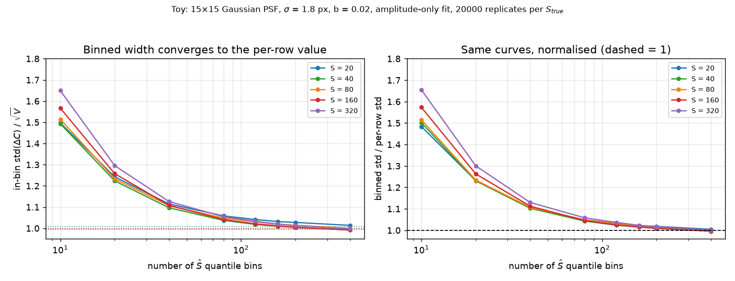
来源:scratchpad/v2/T12/_binfig.py(玩具复现,与 scratchpad/v2/claude_checks/width_cond_resid.py 同一模型、同一种子 20261017;\(S_{true}\) 从 {20, 40, 80, 160, 320} 里独立抽取,每格 20000 次实现)。图为本次重绘,非目录数据。Source: scratchpad/v2/T12/_binfig.py (a toy replay on the same model and the same seed 20261017 as scratchpad/v2/claude_checks/width_cond_resid.py; \(S_{true}\) drawn iid from {20, 40, 80, 160, 320}, 20000 realizations each). The figure was redrawn for this page; it is not catalogue data.
结果。“插入式比条件宽度窄 22–30 %”这个读法撤回了(07 R030,2026-10-17T07:10Z):它是 \(\hat{S}\) 分位数分箱的假象。同一个玩具逐行看,插入式是对的。The result. The reading “the plug-in is 22–30 % narrower than the conditional width” was withdrawn (07 R030, 2026-10-17T07:10Z): it is an artefact of \(\hat{S}\) quantile binning. Row by row in the same toy, the plug-in is right.
来源:cognition-os/07_REVISION_LOG.md R030(撤销 R028 的异议 3);Claude 复现 scratchpad/v2/claude_checks/width_cond_resid.py;T219、T226。Provisional——范围收窄为位置固定、S \(\gtrsim\) 12(R033)。Source: cognition-os/07_REVISION_LOG.md R030 (withdrawing R028’s objection 3); Claude’s replay scratchpad/v2/claude_checks/width_cond_resid.py; T219, T226. Provisional — rescoped to position fixed and S \(\gtrsim\) 12 (R033).
12. 小故事:拟合位置跑到拟合圆边缘时会发生什么12. A Short Story: What Happens When the Fitted Position Wanders to the Edge of the Fitting Circle
问题。拟合器自己选位置。它把源的中心放到离盒子中心很远的地方时,\(\Delta\)C 会怎么变?The question. The fitter picks the position itself. When it puts the source’s centre far from the box centre, what happens to \(\Delta\)C?
先说人话。拟合是在一个小圆里做的(ecut = 15 px 的圆)。模板是画在这个圆里的:源在圆心,光子铺满整个圆。如果拟合器把源挪到圆边上,模板有一半就掉到圆外头去了——那部分光子还在数据里,但模型不允许它们出现在那儿。于是模型比数据"少了一块",\(\Delta\)C 就变小。位置偏得越远,掉出去的越多。还有些源几乎贴着圆壁,那就是一个单独的总体。In plain words first. The fit happens inside a small circle (the ecut = 15 px circle). The template is drawn inside that circle: the source at the centre, its photons spread over the whole circle. If the fitter moves the source to the edge, half the template falls outside the circle — those photons are still in the data, but the model is not allowed to put them there. So the model is “missing a piece” against the data and \(\Delta\)C gets smaller. The further off-centre, the more falls out. And some sources sit almost against the wall; those are a separate population.
图。横轴是拟合位置离中心的距离 \(\hat{r}\)(0–2、2–5、5–10、10–15 px),纵轴是 \(z = (\Delta C - \mu(\hat{S}))/\sqrt{V(\hat{S})}\) 的均值。曲线从近处的约 0 平滑下降到远处 −1.7(DET_ML 6–10)与 −4.0(10–20);在 \(\hat{r}\) \(\gtrsim\) 14.9 px 处还有一群只占 13 % 的行,均值 −3.2——那是贴着圆壁的总体。The picture. The horizontal axis is the fitted offset from the centre \(\hat{r}\) (0–2, 2–5, 5–10, 10–15 px); the vertical axis is the mean of \(z = (\Delta C - \mu(\hat{S}))/\sqrt{V(\hat{S})}\). The curve falls smoothly from about 0 near the centre to −1.7 (DET_ML 6–10) and −4.0 (10–20); at \(\hat{r}\) \(\gtrsim\) 14.9 px there is also a group, only 13 % of the rows, with mean −3.2 — the population hugging the wall.
怎么测的。L0 生产表(我们自己的拟合器)的逐行 \(z = (\Delta C - \mu(\hat{S}))/\sqrt{V(\hat{S})}\),按 \(\hat{r}\) 分箱报告。远行比例按典型 DET_ML 分箱是 28 % / 4.7 %(6–10 / 10–20 窗口);按观测 DET_ML 分箱会给出不同的数(1.015 / 0.997),那是另一种口径。同一个 recert13 试点设计上,典型 DET_ML 格的 std 是 1.34 / 1.29。How it was measured. Per-row \(z = (\Delta C - \mu(\hat{S}))/\sqrt{V(\hat{S})}\) on the L0 production table (our own fitter), reported by \(\hat{r}\) bin. The far fraction by typical DET_ML binning is 28 % / 4.7 % (the 6–10 / 10–20 windows); by observed-DET_ML binning one gets different numbers (1.015 / 0.997), which is a different convention. On the same recert13 pilot design the typical-DET_ML cells give std 1.34 / 1.29.
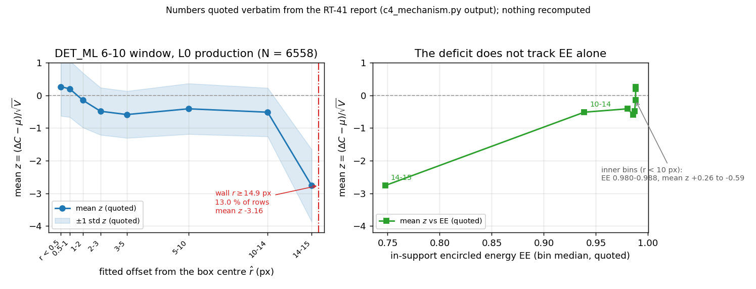
来源:数字逐字引自 RT-41 报告的 c4_mechanism.py 输出(DET_ML 6–10 窗口,N = 6558;reviews/RT-41_triage_claude.md 的 O5),本页只作图、未重算。右图用的 EE 是箱内中位数,不是逐行精确值。Source: the numbers are quoted verbatim from the RT-41 report's c4_mechanism.py output (DET_ML 6–10 window, N = 6558; O5 of reviews/RT-41_triage_claude.md); this page only plots them and recomputes nothing. The EE used in the right panel is the bin median, not a per-row exact value.
结果。L0 在 DET_ML 6–20 的合并 std 1.45 / 1.52 不是一个宽度,是两种总体的混合:近处的行均值约 0,远处的行在插入式下方。所以"look-elsewhere 抬高 \(\Delta\)C"的读法符号相反,已撤回(07 R036)。同样撤回的还有"试点设计里没有这个超出"(07 R039)。L1(emldetect)没有这个问题:用 emldetect 实际得到的背景 BG_MAP_EML 打分,std z 0.95 / 0.975 / 1.00 / 1.02(DET_ML 6–10 / 10–20 / 20–50 / 50–100)、mean z −0.05…−0.07(07 R041;此前用设计水平 b_true 打分得到的 1.02–1.12 与 +0.28…+0.47 已撤回)。R066 把这组格子数值降为历史(格子标签 b_true 不是可观测量):现行说法是可观测 S_eml 箱表——std z 0.94–0.98(DET_ML 1–6)、\(\approx\) 0.95(6–10)、12–20 以上约 1,最低一箱反而宽(1.31);所以 L1 没有 T234 那种低 DET_ML 偏窄。当天深夜 W3 的 codexnim 臂给出了近处行变窄的机制(07 R046,E171/T230):beyond-Fisher 的位置曲率因子 \(\sigma_{ratio}\)(lib/beyond_fisher.py,预测在 \(\pm 5\) % 内),加上它之后近行宽度在 19 个生产格里的 18 个通过;只看 \((\hat{S}, b)\) 的宽度仍描述不了(混合律失败)。The result. L0’s pooled std 1.45 / 1.52 at DET_ML 6–20 is not a width: it is a mixture of two populations, near rows at mean about 0 and far rows below the plug-in. So the reading “look-elsewhere raises \(\Delta\)C” has the opposite sign and was withdrawn (07 R036). Also withdrawn: “the excess is absent in the pilot design” (07 R039). L1 (emldetect) does not have this problem: scored with the background emldetect was actually given (BG_MAP_EML), std z 0.95 / 0.975 / 1.00 / 1.02 (DET_ML 6–10 / 10–20 / 20–50 / 50–100) with mean z −0.05…−0.07 (07 R041; the earlier design-level b_true scoring's 1.02–1.12 and +0.28…+0.47 are withdrawn). R066 demotes this set of cell numbers to history (the cell label b_true is not an observable); the current statement is the observable S_eml bin table — std z 0.94–0.98 at DET_ML 1–6, \(\approx\) 0.95 at 6–10 and about 1 above 12–20, with the lowest bin wide (1.31); so L1 does not show T234's low-DET_ML narrowing. Late that day W3's codexnim arm supplied the mechanism for the near-row narrowing (07 R046, E171/T230): the beyond-Fisher position-curvature factor \(\sigma_{ratio}\) of lib/beyond_fisher.py (predicted within \(\pm 5\) %), with which the near-row width passes in 18 of 19 production cells; the width given \((\hat{S}, b)\) alone is still not described (the mixture law fails).
来源:T228(Provisional);07 R036、R039;reviews/RT-40、reviews/RT-41_triage_claude.md(O3–O5,机制未复现,数字在 c4.log)。Source: T228 (Provisional); 07 R036, R039; reviews/RT-40, reviews/RT-41_triage_claude.md (O3–O5; the mechanism was not replayed, the numbers are in c4.log).
9. 一页总结9. One-Page Summary
| 概念Concept | 一句话In One Sentence | 公式Formula |
|---|---|---|
| 泊松分布Poisson distribution | 光子计数的基本涨落The basic fluctuation in photon counts | P(Y=k) = λᵏe^(−λ)/k! |
| PSFPSF | 点源光子的空间分布Spatial distribution of a point source's photons | μᵢ = b + S·Pᵢ |
| Cash 统计量Cash statistic | 泊松似然的 −2 倍对数−2×log of the Poisson likelihood | C = 2Σ(μ − Y ln μ) |
| ΔCΔC | "有源 vs 没源"的似然比"Source vs no-source" likelihood ratio | ΔC = C_null − C_min |
| Wilks 定理Wilks' theorem | 大样本极限 ΔC ~ χ²(ν)Large-sample limit ΔC ~ χ²(ν) | ν = 自由参数个数ν = number of free parameters |
| DET_MLDET_ML | ΔC 的非线性变换,目录用的检测量Nonlinear transform of ΔC, the catalogue's detection quantity | DET_ML = −ln Q(ν/2, ΔC/2) |
| 铁律Iron Rule | 不许按 ML 切样本No ML-based sample cuts | 条件化 (Ŝ, b),残差在 ΔC 空间condition on (Ŝ, b); residuals in ΔC space |
| Eddington 偏差Eddington bias | 暗源多 + 涨落 ⇒ 测得的偏亮Faint sources dominate + scatter ⇒ measured fluxes biased high | E[S | Ŝ] < Ŝ(暗端)E[S | Ŝ] < Ŝ (faint end) |
下一页讲这个项目的历史:这些概念是怎么一个一个被逼出来的。The next page tells the project's History: how these concepts were forced out one by one.