E163 项目手册 · 中文正文，术语首次出现保留英文E163 project handbook · English version (Chinese is the default)

这个项目为什么存在Why This Project Exists

这一页回答 3 个问题：项目在做什么、为什么值得做、以及一个数字看懂它现在的位置。假设你是一年级物理本科生：会微积分、懂一点概率、会一点 Python，不知道什么是泊松似然。This page answers 3 questions: what the project does, why it is worth doing, and one number that shows where it stands. We assume you are a first-year physics undergraduate: you know calculus, some probability, some Python, and nothing about the Poisson likelihood.

这个项目在做什么What the Project Does

X 射线望远镜 XMM-Newton 巡天时，软件 emldetect 给每个候选源输出两个数：When the X-ray telescope XMM-Newton surveys the sky, the software emldetect outputs two numbers for each candidate source:

Ŝ（fitted flux）：测得的流量； (fitted flux): the measured flux;
DET_ML（detection likelihood，检测似然）：这个信号有多不像背景涨落。 (detection likelihood): how unlike a background fluctuation this signal is.

目录（catalogue）用 DET_ML ≥ 6 来决定哪些源"算数"。但 DET_ML 本身是一个随机数：同一个源再测一次，DET_ML 会变。这个项目要回答的问题是：给定你能观测到的量（Ŝ、背景 b、位置），DET_ML 背后的统计量 ΔC 应该服从什么分布？有了这个分布，就能回答目录使用者真正关心的问题：完备度（completeness）是多少？测得的流量偏亮了多少（Eddington bias）？The catalogue uses DET_ML ≥ 6 to decide which sources "count". But DET_ML itself is a random number: observe the same source again and DET_ML will change. The question this project answers is: given the quantities you can observe (Ŝ, background b, position), what distribution should ΔC — the statistic behind DET_ML — follow? With that distribution one can answer what catalogue users actually care about: what is the completeness? How much too bright are the measured fluxes (Eddington bias)?

完整的故事从The full story starts on the 物理与统计Physics & Statistics一页讲起。 page.

为什么值得做Why It Is Worth Doing

大多数目录源都挤在阈值附近。Most catalogue sources crowd near the threshold.4XMM 目录的入选线是 DET_ML = 6，而最暗的、数量最多的源恰好分布在这个阈值上方一点点。这里的统计规律最不"高斯"，也最难算。The 4XMM catalogue's acceptance line is DET_ML = 6, and the faintest, most numerous sources sit just above it. The statistics there are the least "Gaussian" and the hardest to compute.
XMM 官方文档承认这是空白。The official XMM documentation admits this gap.灵敏度图文档明确说"没有简单的泊松模型能匹配 emldetect 的检测似然行为"，建议用蒙特卡洛校准。本项目就是要把这个空白填上一个可计算、可验证的公式（来源：GOAL.md §1.4）。The sensitivity-map documentation states plainly that "no simple Poisson model matches the detection-likelihood behaviour of emldetect" and recommends Monte Carlo calibration. This project fills that gap with a computable, testable formula (Source: GOAL.md §1.4).
错了会出什么问题：What goes wrong if it is not understood:把背景涨落当成源（假源）、漏掉真源（完备度）、以及暗源被系统性地测得太亮（Eddington bias，见background fluctuations counted as sources (false sources), real sources missed (completeness), and faint sources systematically measured too bright (Eddington bias; see the 动画animation）。).

一个数字看懂全项目One Number Explains the Whole Project

项目从 2026-03 走到今天，最近的一个里程碑是（来源：cognition-os/04_DECISION_LOG.md，2026-10-13 03:30 条目）：The project has run from 2026-03 to today; the most recent milestone is (Source: cognition-os/04_DECISION_LOG.md, 2026-10-13 03:30 entry):

不用任何在目录上拟合的参数，只靠物理推导，孤立点源在检测阈值附近（DET_ML 6–10）的 ΔC 均值偏差从 v1 基线的 0.60σ 降到 0.13σ（基准计分器的噪声校正 A1，benchmark/leaderboard_v2.json，C-iso 层），与一个拟合了 6 个参数的经验模型（0.125σ，样本内）统计上打平。Without any parameter fitted on the catalogue, from physics alone, the ΔC mean bias of isolated point sources near the detection threshold (DET_ML 6–10) fell from the v1 baseline of 0.60σ to 0.13σ (the benchmark scorer's noise-corrected A1, benchmark/leaderboard_v2.json, C-iso layer), statistically tied with a 6-parameter empirical model (0.125σ, in-sample) — No significant difference.

但注意：2026-10-13 的 T11_020 评审随后发现，带来这个改善的二维位置损失在三个 ML 窗口上并不平坦——它不是最终的闭合项。当前前沿条目的分数仍然成立，但"均值问题已解决"这句话要等联合拟合损失的正确形式定下来才能说。见But note: the T11_020 review later on 2026-10-13 found that the two-dimensional position loss behind this improvement is not flat across the three ML windows — it is not the final closing term. The current front entries' scores still stand, but "the mean problem is solved" must wait until the correct form of the joint-fit loss is settled. See the 工作台的未解决问题表workbench open-problems table。.

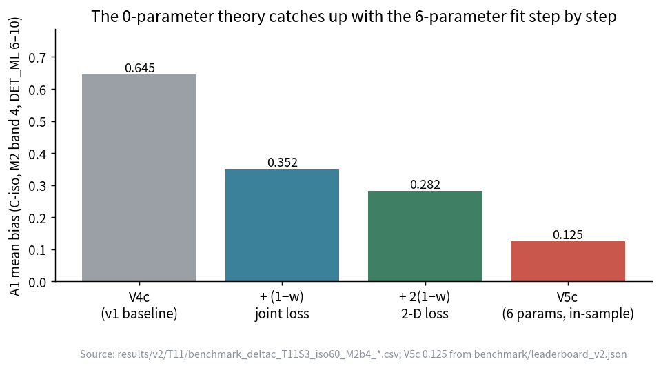
A1 均值偏差逐步下降的柱状图 — 逐箱加权 A1 口径（T11 分箱表，与上图基准计分器口径不同）：v1 基线 0.604 → 加联合拟合损失 0.300 → 加二维位置损失 0.156；红色是样本内的 6 参数模型 0.125（只作参考）。两种口径的对比正是评审指出的易混点——引用时先说用哪一种。Per-bin count-weighted A1 estimator (T11 bin table; a different estimator from the scorer's value above): v1 baseline 0.604 → + joint-fit loss 0.300 → + two-dimensional position loss 0.156; red is the in-sample 6-parameter model at 0.125 (reference only). The contrast between the two estimators is exactly the confusion the review flagged — name the estimator before quoting it.

来源：results/v2/T11/benchmark_deltac_T11S3_iso60_M2b4_*.csv（逐箱口径）；benchmark/leaderboard_v2.json（基准计分器口径）。Source: results/v2/T11/benchmark_deltac_T11S3_iso60_M2b4_*.csv (per-bin estimator); benchmark/leaderboard_v2.json (scorer estimator).

怎么分清“真的物理”和“我们自己的仪器”How to Tell Real Physics from Our Own Instrument

一个学生会问：你说低计数端的中心项偏高了，那会不会只是你的模板和拟合器把光加错了？这是个好问题，而且它有标准的答法。A student asks: you say the centre term is biased high at low counts — could that just be your template and fitter adding the light up wrong? That is a good question, and it has a standard answer.

物理图像。一台 X 射线望远镜看到的不是“一个点源的流量”这个抽象数字，而是一张像素图：仪器用一个点扩散函数（PSF）把每个光子摊到几个像素上，背景在逐像素变化，读出还有噪声。要问“这个源比检测阈值亮多少”，我们必须先把模板（PSF 的形状）放在图上、把背景减掉、再把模板里的光加起来。每一个环节都可能引入系统项：PSF 栅格取在哪、背景按什么律、模板族怎么参数化、拟合器怎么搜索——而它们恰恰在源很暗、只有几十个光子时最重要，因为那时“信号的形状”最不确定。The physical picture. An X-ray telescope does not see “the flux of a point source” as an abstract number; it sees a pixel image: the instrument spreads each photon over a few pixels with a point-spread function (PSF), the background varies pixel by pixel, and the readout adds noise. To ask “how much brighter is this source than the detection threshold” we must first place a template (the PSF shape) on the image, subtract the background, and add up the light inside the template. Every one of those steps can introduce a systematic: where the PSF raster sits, what background law is used, how the template family is parameterised, how the fitter searches — and they matter most precisely when the source is faint, with only tens of photons, because then “the shape of the signal” is the least certain.

测量怎么回答。办法是造一个匹配对照：用一模一样的 PSF 栅格、一模一样的掩膜、一模一样的背景律、一模一样的抖动，在同一个位置上再造一批“源”，然后用同一条流水线去测它。如果流水线本身有系统项，对照那一侧也会同样偏；两边相减，剩下的就是流水线内部的差异（模板族、拟合器）。反过来，如果换一个真正不同的仪器（不同波段、不同 PSF）做对照，相减就混进了仪器差异，什么也证明不了。How the measurement answers. Build a matched control: generate another batch of “sources” with the identical PSF raster, the identical mask, the identical background law and the identical jitter, at the same position, then measure it with the same pipeline. If the pipeline itself has a systematic, the control side is biased the same way; subtracting the two leaves only what differs inside the pipeline (the template family, the fitter). Conversely, if you use a genuinely different instrument (a different band, a different PSF) as the control, the subtraction mixes in the instrument difference and proves nothing.

结果（来源：07 R082、R084、R085，均已复算；归因由 R087 撤回）。在匹配对照下，L0 的低计数中心项超额依然存在，但它衡量的不是 emldetect 的物理，而是 L0 这条流水线自己的性质——72/28 的归因（模板族对 plug-in 均值）已被 R087 撤回：把同一批对照图用 FFT 模板族与 v2t1 重新拟合，只补上 0–27 % 的差距，超额的成因开放。按可观测的 \(\hat{S}\) 分箱，差距是 \(\hat{S}\) < 4 处 +0.389、\(\hat{S}\) 4–11 处 +0.14–0.18、\(\hat{S}\) \(\geq\) 11 处 +0.058 \(\pm\) 0.007，到高计数锚处约 0。白话：这个项目最重要的方法论一课——当你怀疑一个效应是自己的仪器造成的，不要换一台更“干净”的仪器去比，而要造一个逐项相同的对照，让唯一变化的东西自己浮出来。Result (sources: 07 R082, R084, R085, all replayed; the attribution is withdrawn by R087). Against the matched control the L0 low-count centre excess is still there, but what it measures is not emldetect physics — it is a property of the L0 pipeline itself; the 72/28 split (template family against plug-in mean) is withdrawn by R087: refitting the same control images with the FFT family and v2t1 closes only 0–27 % of the gap, and the excess's cause is open. In observable \(\hat{S}\) bins the gap is +0.389 at \(\hat{S}\) < 4, +0.14–0.18 at \(\hat{S}\) 4–11 and +0.058 \(\pm\) 0.007 at \(\hat{S}\) \(\geq\) 11, reaching about 0 at the high-count anchor. In plain words: the project's most important methodological lesson — when you suspect an effect is caused by your own instrument, do not compare against a “cleaner” instrument; build a control that matches item by item and let the one thing that varies stand out by itself.

主线回到 emldetect 的理由后来被 R086 改写：L1 的宽度偏窄（std z 0.946 [0.937, 0.955] 于 DET_ML 6–10）可以用同一个 penalty 错配机制解释——用合并估计量，L1 的错配在 DET_ML 6–10 是 +1.19 % [+1.03, +1.35]（R083 的 −0.14 % 是逐格比值的平均，已被 R086 推翻），解释了箱内宽度缺口的 0.89 [0.84, 0.93]（预测 std z 0.919，实测 0.918）。所以同一个 \(V_{3p}\) 机制同时决定 L0 与 emldetect 的宽度；任务 0b（同图同打分的配对实验）已完成（R089，已复算）：emldetect 与 L0 高计数一致，DET_ML ≲ 7 处 emldetect 中心比 L0 低 0.16–0.53 z、宽 0.05–0.14——L0 的低计数中心项超额不是 emldetect 的性质，单图 emldetect 规律必须在 emldetect 输出上建立。The reason the main line returned to emldetect was later rewritten by R086: the L1 narrow width (std z 0.946 [0.937, 0.955] at DET_ML 6–10) can be explained by the same penalty-mismatch mechanism — with pooled estimators the L1 mismatch at DET_ML 6–10 is +1.19 % [+1.03, +1.35] (R083's −0.14 % was a mean of per-cell ratios, reversed by R086), explaining 0.89 [0.84, 0.93] of the within-cell width deficit (predicted std z 0.919, observed 0.918). The same \(V_{3p}\) mechanism carries both the L0 and the emldetect widths; task 0b (the paired same-images-same-scoring run) is completed (R089, replayed): emldetect and L0 agree at high counts and at DET_ML ≲ 7 emldetect's centre is 0.16–0.53 z lower and its width 0.05–0.14 larger than L0 — the L0 low-count centre excess is not an emldetect property, and the single-image emldetect law must be built on emldetect output.

怎么读这本手册How to Read This Handbook

工作台Workbench——一屏看懂项目、目标、未解决问题和计划；日常从这里开始。 — the project, its objectives, open problems and the plan in one screen; start here daily.
物理与统计Physics & Statistics——从光子计数讲到 DET_ML，每步一个算例，五个动画。 — from photon counting to DET_ML, one worked example per step, five animations.
历史History——项目怎么走到今天，哪些路走通了，哪些是死胡同。 — how the project got here, which paths worked, which were dead ends.
基准设计Benchmark Design——现在评价一个理论好坏的规则。 — the current rules for judging a theory.
现状Current State——已确立、进行中、开放的完整清单。 — the full list of what is established, running, and open.
动手指南Handbook——不用 AI、自己动手继续这个项目的操作手册。 — the operations manual for continuing this project by hand, without AI.
词汇表Glossary——所有符号和缩写，以及关键文献。 — every symbol and acronym, plus the key papers.

建议（未经评审）：第一次读按上面的顺序通读一遍，之后把Suggestion (not reviewed): read through in the order above the first time, then keep the 工作台Workbench当作日常首页。所有命令都已在真实代码上核对过。 as your daily home page. Every command has been checked against the real code.